OLS is the conventional method for estimating the parameters in the linear regression model. The LS in OLS stands for Least Squares, and the O just means that we are talking about the Ordinary form of least squares rather than a more elaborate variant.
Least squares is a criterion for comparing estimates of \(\beta\) and identifying the best one. Under least squares, the best estimates are the estimates that minimize the sum of the squared errors, or squared residuals. The error is the difference between the predicted value of the outcome (\(\hat{y}\)) given the estimates and the observed value of the outcome (\(y\)).
Sometimes this is talked about with the language of a cost function. The idea is to think of errors as being costly, and so the preferred estimates are those that minimize cost. OLS, then, involves defining the “cost” of an error as equal to the magnitude of the error squared.
Example
To make the least squares criterion concrete, we are going to find the best \(\hat{\beta}\) ourselves, by hand, without asking the computer to fit the model. This is worth doing because it shows exactly what OLS is minimizing — and because later in the course we will encounter models that do not have a tidy analytic solution, where understanding an alternative approach–iterative estimation–becomes essential.
Is the critical appraisal of a movie associated with how much money it makes? We can look at data on 609 movies released between 2008 and 2012. Our explanatory variable \(\texttt{rtscore}\) is the film’s score on Rotten Tomatoes (0-100 scale, based on critics’ reviews). Our outcome \(\texttt{usgross}\) is US gross box-office revenue in millions of dollars.
For the purposes of this exercise, I will center both of these variables, meaning that I will subtract the mean from each variable, so that the new mean of the variable is 0. (More information on how to do this in Stata or R is at the end of this page.)
Centering a variable does not change its standard deviation. Centering the explanatory variable and outcome does not affect the slope of the ensuing regression line. What centering does do in this case is change the constant of the regression model so that it is 0.
We do this so that the regression model has only one parameter: the slope, or the change in revenue associated with a one-unit change in Rotten Tomatoes score.
Aside: Why does centering the variables make the constant zero? In OLS, the regression line always passes through the centroid of the data. In our case, the regression line must pass through the point where the mean of \(\texttt{rtscore}\) intersects with the mean of \(\texttt{usgross}\). If we center both variables, then the regression line must pass through the point at which \(x\) and \(y\) are both 0. The intercept in the regression model is the predicted value of \(y\) when \(x\) is 0, so if both variables are centered the constant is 0.
where \(\widehat{\texttt{usgross}}_i\) is our \(\hat{y}\).
So what is \(\hat{\beta}\)? This is what we will now figure out, by ourselves, without having the computer fit the model for us.
What we want is the \(\hat{\beta}\) that minimizes the sum of squared errors. For any candidate value of \(\hat{\beta}\), we can calculate the sum of squared errors.
\[
\sum_{i=1}^{N} (\hat{y}_i - y_i)^2
\]
For example, say the candidate answer for \(\hat{\beta}\) that we want to try is .5. We could follow these steps:
Calculate \(\hat{y}_i = .5 \times \texttt{rtscore}_i\) for every observation
::: {.statacode}
. drop yhat error error_squared

. gen yhat = 1*rtscore

. gen error = yhat - usgross

. gen error_squared = error * error

. quietly summarize error_squared

. display r(sum) // after summarize, provides total sum of variable
3659125.9
:::
The sum of the squared errors is now 3659126, which is smaller than the previous sum. So, by the least squares criterion, \(\beta\) = 1 is a better estimate than \(\beta\) = .5.
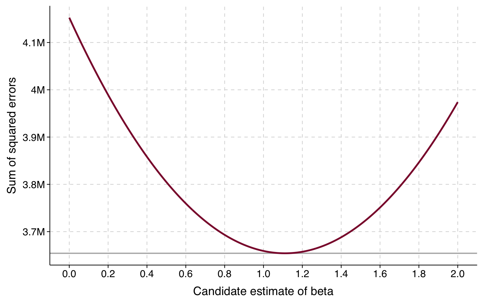
We can try a bunch of different guesses and plot the result. Here is what we get when we plot the results between 0 and 2:
Click for R code that draws plot
betas <-seq(0, 2, by =0.005)sse <-sapply(betas, function(b) sum((b * df$rtscore - df$usgross)^2))sse_df <-data.frame(beta = betas, sse = sse)ggplot(sse_df, aes(x = beta, y = sse)) +geom_hline(yintercept =min(sse), color ="gray70", linewidth =0.7) +geom_line(color ="#8B1538", linewidth =1) +scale_x_continuous(breaks =seq(0, 2, 0.2)) +scale_y_continuous(labels =function(x) paste0(round(x /1e6, 1), "M")) +labs(x ="Candidate estimate of beta", y ="Sum of squared errors") +theme_tula()
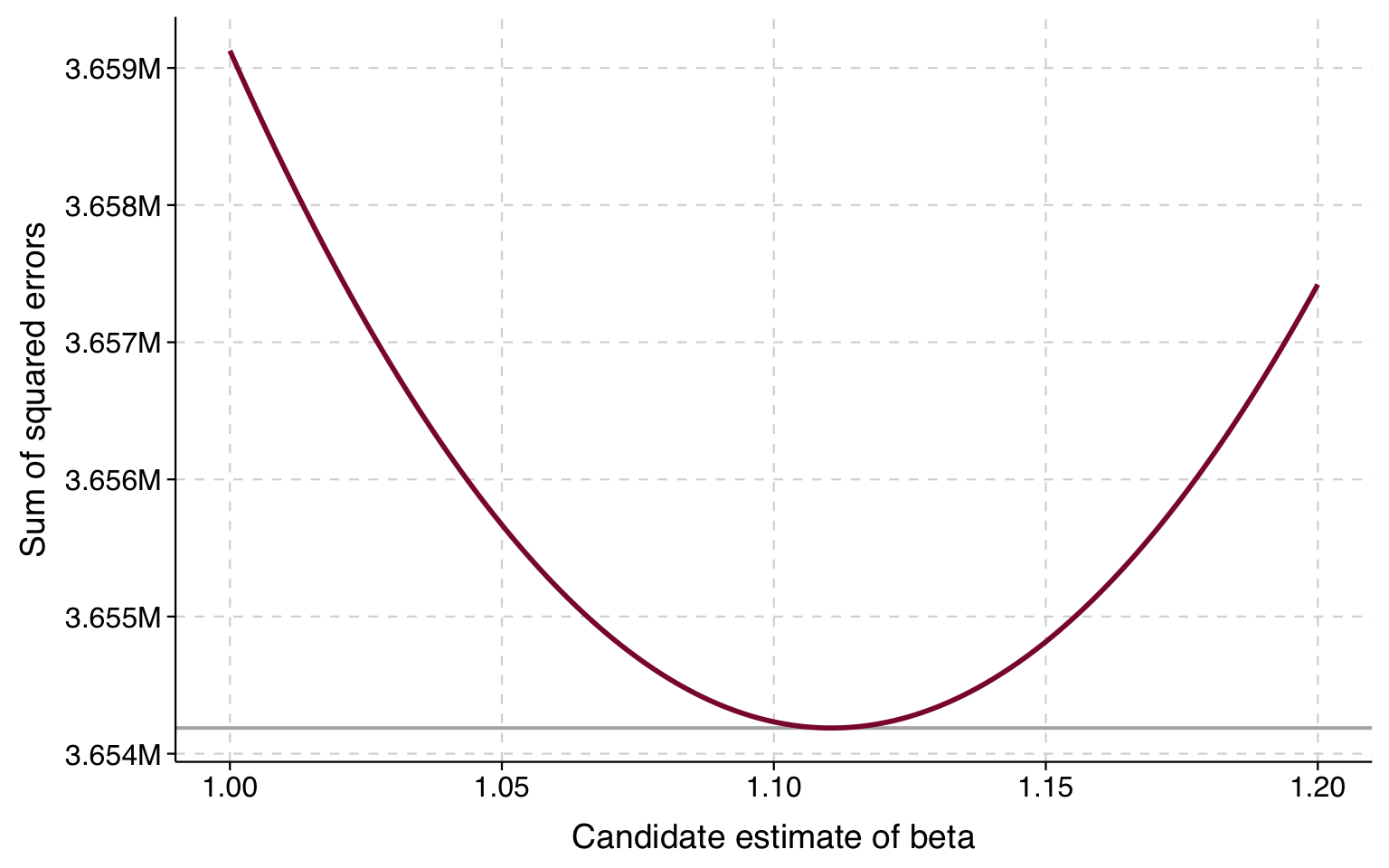
The lowest sums of squares look like they are between 1 and 1.2. So we can plot guesses in this range and look again:
Click for R code that draws plot
betas2 <-seq(1, 1.2, by =0.001)sse2 <-sapply(betas2, function(b) sum((b * df$rtscore - df$usgross)^2))sse_df2 <-data.frame(beta = betas2, sse = sse2)ggplot(sse_df2, aes(x = beta, y = sse)) +geom_hline(yintercept =min(sse2), color ="gray70", linewidth =0.7) +geom_line(color ="#8B1538", linewidth =1) +scale_x_continuous(breaks =seq(1, 1.2, 0.05)) +scale_y_continuous(labels =function(x) paste0(format(round(x /1e6, 3), nsmall =3), "M")) +labs(x ="Candidate estimate of beta", y ="Sum of squared errors") +theme_tula()
The value of \(\beta\) corresponding to the lowest sum of squares appears to be just over 1.1. Now let’s fit the model and show that it corresponds to the results from OLS:
A one-point increase in a film’s Rotten Tomatoes score is associated with a $1.11 million increase in US gross box office revenue.
Analytic and iterative solutions
When you fit an OLS model in a stats package, the stats package is not following the process we used above to find \(\beta\). This is because in OLS there is an analytic solution for \(\beta\). Instead, it solves for the \(\mathbf{\beta}\) that minimize the sum of squared errors using the following matrix algebra operation:
If you take a course on OLS regression taught in matrix algebra, this formula is seared into your brain forever. I am sure there are folks out there with it tattooed.
But, as we showed with our simple example, you don’t need to use this analytic solution to figure out the least squares \(\beta\) to whatever level of precision you care about. Because least squares tells you how to compare possible \(\beta\) values and decide which is better, you can find the answer iteratively, meaning that you try out different estimates and compare them using your criterion and progressively zero in on the best estimates.
What’s great about this is that other models involve estimation strategies that do not have analytic solutions but can be solved iteratively. The way that statistics packages find solutions iteratively is not as clunky as what we did above; instead, there are methods for finding the optimum with far fewer (and much smarter) guesses.
Bonus: How to center a variable
In Stata, if you summarize a variable, then it will temporarily store the mean of that variable as \(\texttt{r(mean)}\). You can use that to center a variable, like this:
. summarize usgross rtscore

    Variable |        Obs        Mean    Std. Dev.       Min        Max
-------------+---------------------------------------------------------
     usgross |        609    75.81977    82.64335   2.778752   760.5076
     rtscore |        609    47.19212    25.78123          0         99

. quietly summarize usgross // suppresses output

. replace usgross = usgross - r(mean)
(609 real changes made)

. quietly summarize rtscore // suppresses output

. replace rtscore = rtscore - r(mean)
variable rtscore was byte now float
(609 real changes made)

. summarize usgross rtscore

    Variable |        Obs        Mean    Std. Dev.       Min        Max
-------------+---------------------------------------------------------
     usgross |        609   -3.67e-08    82.64335  -73.04102   684.6879
     rtscore |        609   -2.22e-07    25.78123  -47.19212   51.80788
More generally, Stata has various commands that write results to \(\texttt{r()}\), and the results stored by one command in \(\texttt{r()}\) are kept there until another command writes anything to \(\texttt{r()}\), at which point whatever was put there by the last command is erased. At any point, you can see what is being stored in \(\texttt{r()}\) by typing \(\texttt{return list}\).
Here are a couple of ways of centering a variable in R. One uses the \(\texttt{scale()}\) function and the other uses the \(\texttt{mean()}\) function:
# using scale()df$usgross <-scale(df$usgross, scale =FALSE)[,1]# using mean()df$rtscore <- df$rtscore -mean(df$rtscore)
With R’s \(\texttt{scale()}\) function, we need to specify \(\texttt{scale=FALSE}\) because \(\texttt{scale=TRUE}\) (the default) will standardize the variable, not just centering it but rescaling it so that the standard deviation is 1.