Least squares and the normal distribution
Least squares
When we fit data by least squares, each observation has an error, for the predicted value minus the observed value: \(\hat{y_i} - y_i\). In OLS, squared errors define the “badness” of a set of estimates. Least squares minimizes the sum of the squared errors over all the observations: \(\sum_{i=1}^N(\hat{y_i} - y_i)^2\).
By squaring the error, the badness associated with a set of errors does not just get bigger as the errors increase, but the penalty gets bigger by bigger amounts. As a result, for example, OLS would prefer to fit 1000 observations with a absolute error of 1, then to fit 999 observations perfectly (error = 0) but 1 observation with an absolute error of 40. (Even though the sum of the absolute errors is much worse – 1000 vs. 40 – the sum of the squared errors is better – 1000 vs. 1600).
We can graph the size of the squared error by the size of the error here:
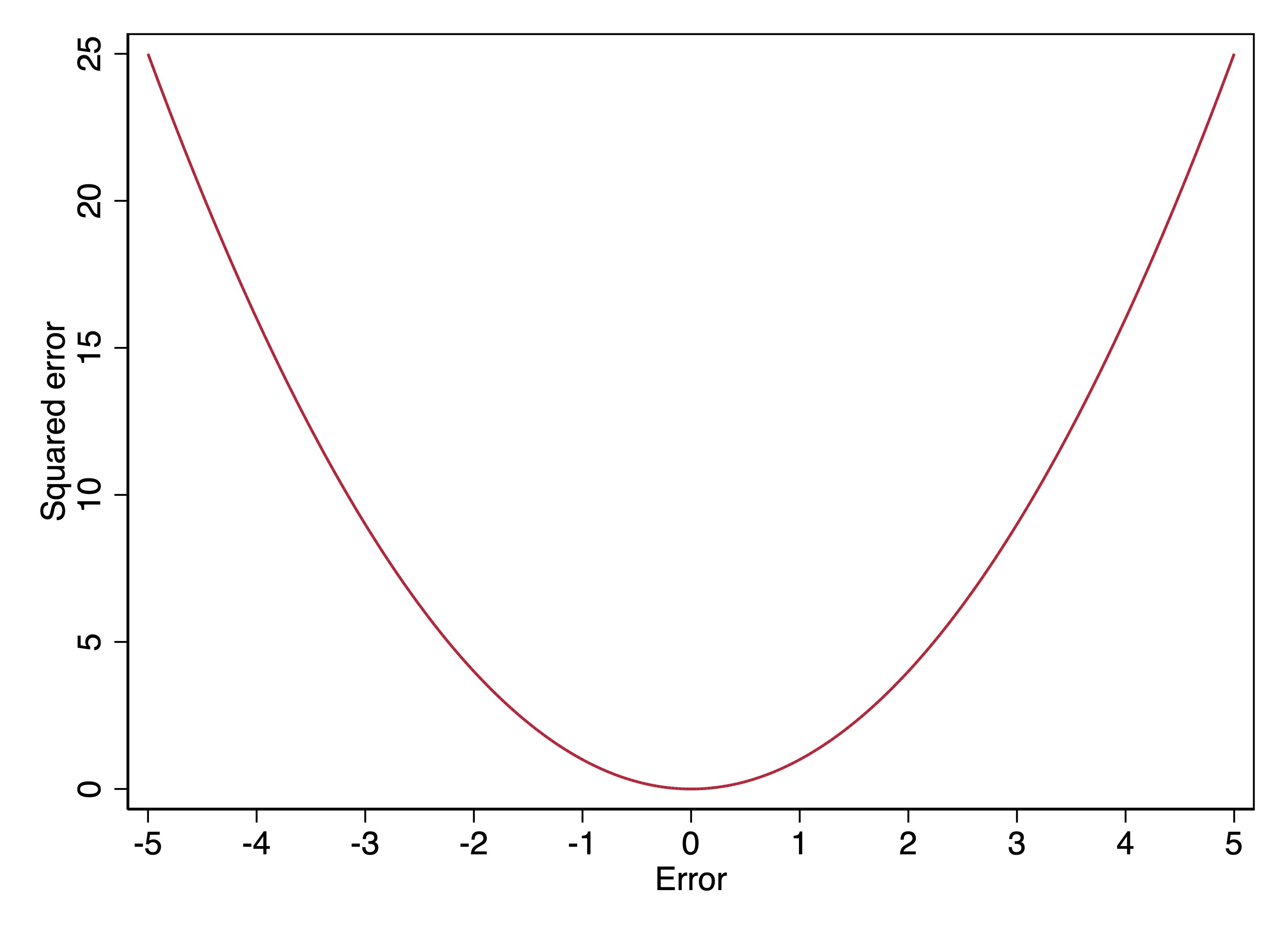
In terms of the values plotted on the y- vs. x-axis here, this graph just \(y=x^2\), which in math is often referred to as the square function.
The standard normal distribution
You are all familiar with the normal distribution. The standard normal distribution is a normal distribution with a mean of 0 and a standard deviation of 1. Here is the standard normal distribution:
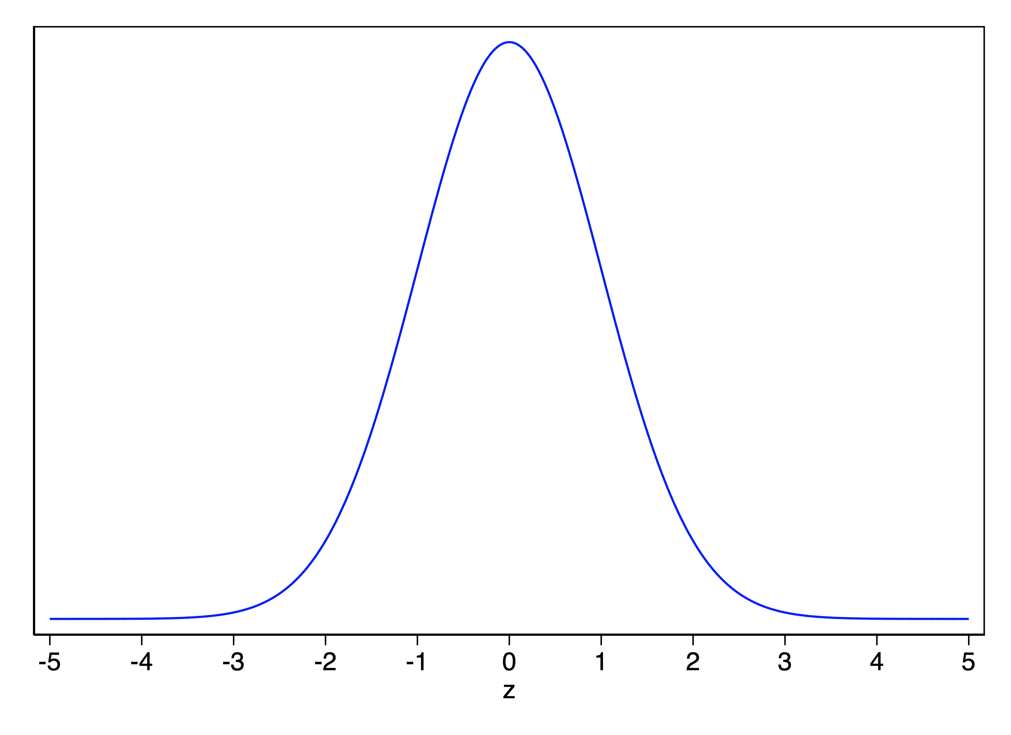
The shape of the standard normal distribution is given by:
\[ y = \exp\left(-\frac{x^2}{2}\right) \]
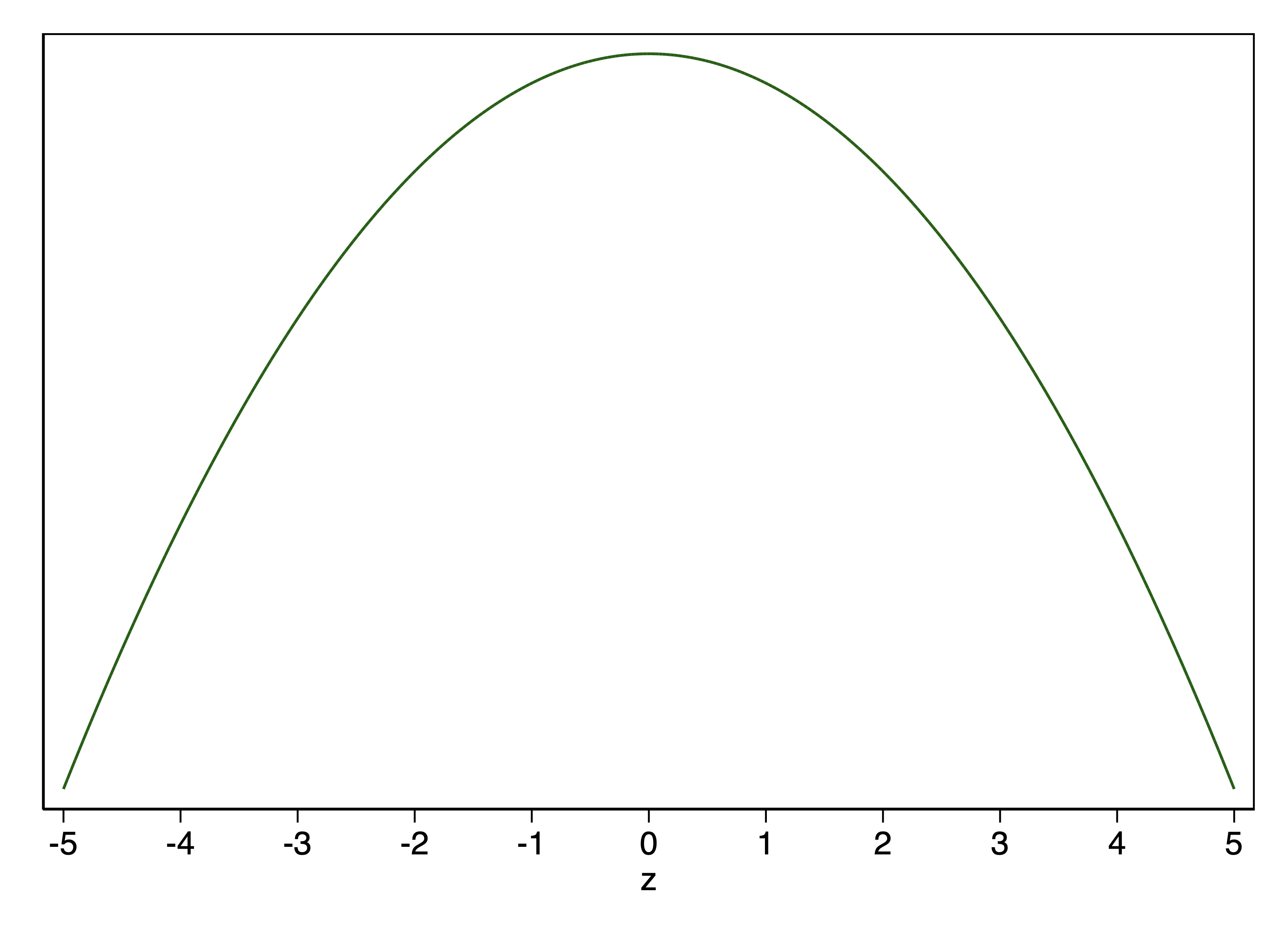
If we log both sides of this equation, we get:
\[ \begin{align} \ln(y) &= -\frac{x^2}{2} \\ \\ &= -\frac{1}{2}(x^2) \end{align} \]
This means that the log of the shape of the standard normal distribution is just the outcome of a square function times -. The negative sign there is maybe the most important bit conceptually, as it means that log of the shape of the standard normal distribution has its maximum at x = 0, whereas for the square function its minimum is x = 0.
Why this is important is that it means when we minimize least squares, we are maximizing something with respect to the log of the shape of the normal distribution. Instead of selecting \(\beta\) on the basis of what minimizes the sum of least squares, we could selecting \(\beta\) in terms of what maximizes the sum of logged values of the normal distribution, and we would get exactly the same \(\beta\).
Right now, it is fair to wonder why one would want to do this, as it seems like we are swapping something familiar for something more complicated. The reason is that soon we will move to problems in which the idea of motivating estimation by least squares is no longer an option. But, if we understand what makes least squares estimates such a good approach to estimating conditional means in the context of well-behaved continuous outcomes, we will have a rationale that we can apply to a much broader range of problems.
Elaboration: If we multiply the right side of the above formula for the standard normal distribution by \(\frac{1}{\sqrt{2\pi}}\), then the total area under the curve is 1. Why this is the case would take us too far afield. But, because the area under the curve is 0, this rescaled function is then the probability density function (PDF) of the standard normal distribution. The use of areas of a PDF to represent probabilities is something we will be doing later. But now, anything with \(\frac{1}{\sqrt{2\pi}}\) is just a distraction. When we take the step of logging both sides of the equation, this becomes \(-\ln\frac{1}{\sqrt{2\pi}}\) on the right side, which is a constant. So it does not change the result that minimizing the sum of least squares maximizes the sum of logged densities from the normal distribution.