Normally distributed errors in linear regression
Above we wrote the linear regression model as:
\[ y_i = \mathbf{x}_i\mathbf{\beta} + \mathbf{\varepsilon}_i \]
With our running example in which the outcome is height and the explanatory variables are sex (binary), age, and a five-category race/ethnicity variable, we can write this as follows:
\[ \begin{split} \textrm{Height}_i = \enspace & \beta_0 + \beta_1(\texttt{male}_i) + \beta_2(\texttt{age}_i) + \beta_3(\texttt{oth_hisp}_i) \\ & + \beta_4(\texttt{nonh_white}_i) + \beta_5(\texttt{nonh_black}_i) + \beta_6(\texttt{nonh_other}_i) \\ & + \varepsilon_i \end{split} \]
As a model of the height generating process, the model presents an individual’s height as generated by an additive combination of a systematic component and a stochastic component.
- The systematic component relates an individuals height to their sex, age, and race/ethnicity through coefficients attached to their characteristics.
- The stochastic component says that, after the systematic component is taken into account, the remainder of height can be usefully treated as a random draw from a statistical distribution. We are not claiming that height is otherwise completely random, just maybe that it can be treated as such without distorting whatever is the practical purpose of the model (e.g., estimates of the coefficients).
The conventional assumption about the error distribution for a linear regression model is that the errors are normally distributed. As I indicated before, violation of this assumption does not mean that the coefficients are biased.
The normal distribution does have some nifty properties when it comes to representing error. If you imagine a process where error is produced as a result of a large bunch of small perturbations that are equally likely to push an observation toward or away from the mean by a given amount, the result is a normal distribution. You can buy toys that are based upon this principle, or see demonstations of it in science museums.
The simplest form of the assumption is normally distributed errors in the linear regression model is that the error term of each observation is independent and identically distributed as normal. This means that the error for a given observation:
- Does not depend on the value of the error drawn for any other observation.
- Does not depend on the observations values of the explanatory variables.
There are whole swaths of regression methods concerning what to do in the face of the violation of these assumptions (especially #1), but we are not concerning ourselves with that here.
The standard normal distribution
When a normal distribution has a mean 0 and standard deviation of 1, it is called the standard normal distribution.
But a normal distribution can have any mean and any standard deviation. It the standard deviation is greater than 1 it will be shorter and more stretched out than the standard normal – and if it is less than 1 it will be less spread out, but it will have the same fundamental shape.
In OLS, a key assumption is that the mean of the error term is 0, while the standard error of the error term is not assumed to be anything–rather, it is given by the RMSE (which we discussed earlier.
If you divide the residuals (errors) from regression by the RMSE, they will have a standard deviation of 1. The residual divided by the RMSE is called the standardized residual, and it can be useful because it means one can talk about the magnitude of error in a way that is independent from the variable itself. For example, a residual of 5 could be big or small depending on the scale of the dependent variable – if we were talking about annual income in dollars, an error of only 5 dollars would be impressively tiny, whereas a standardized residual of 5 is always big (if the errors are normally distributed, one would only expect to observe a residual that larger or larger in about 1 in 1.7 million observations).
The normal distribution and the likelihood of error
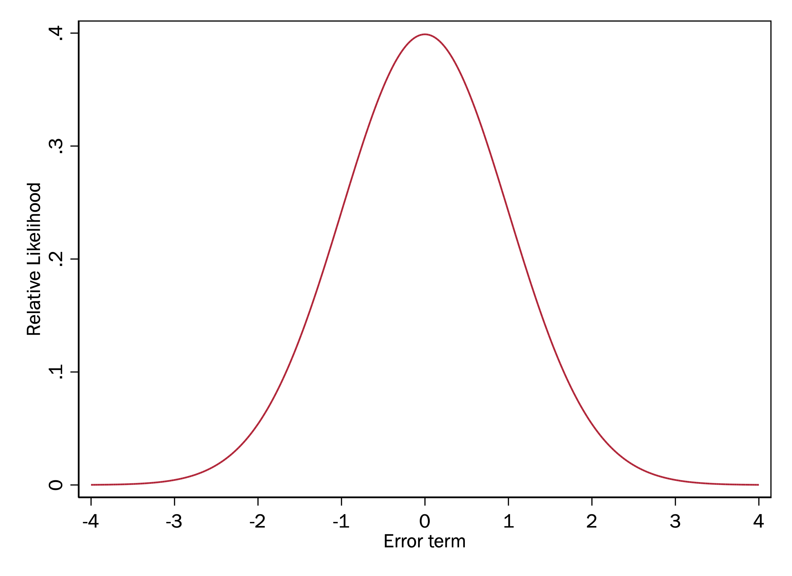
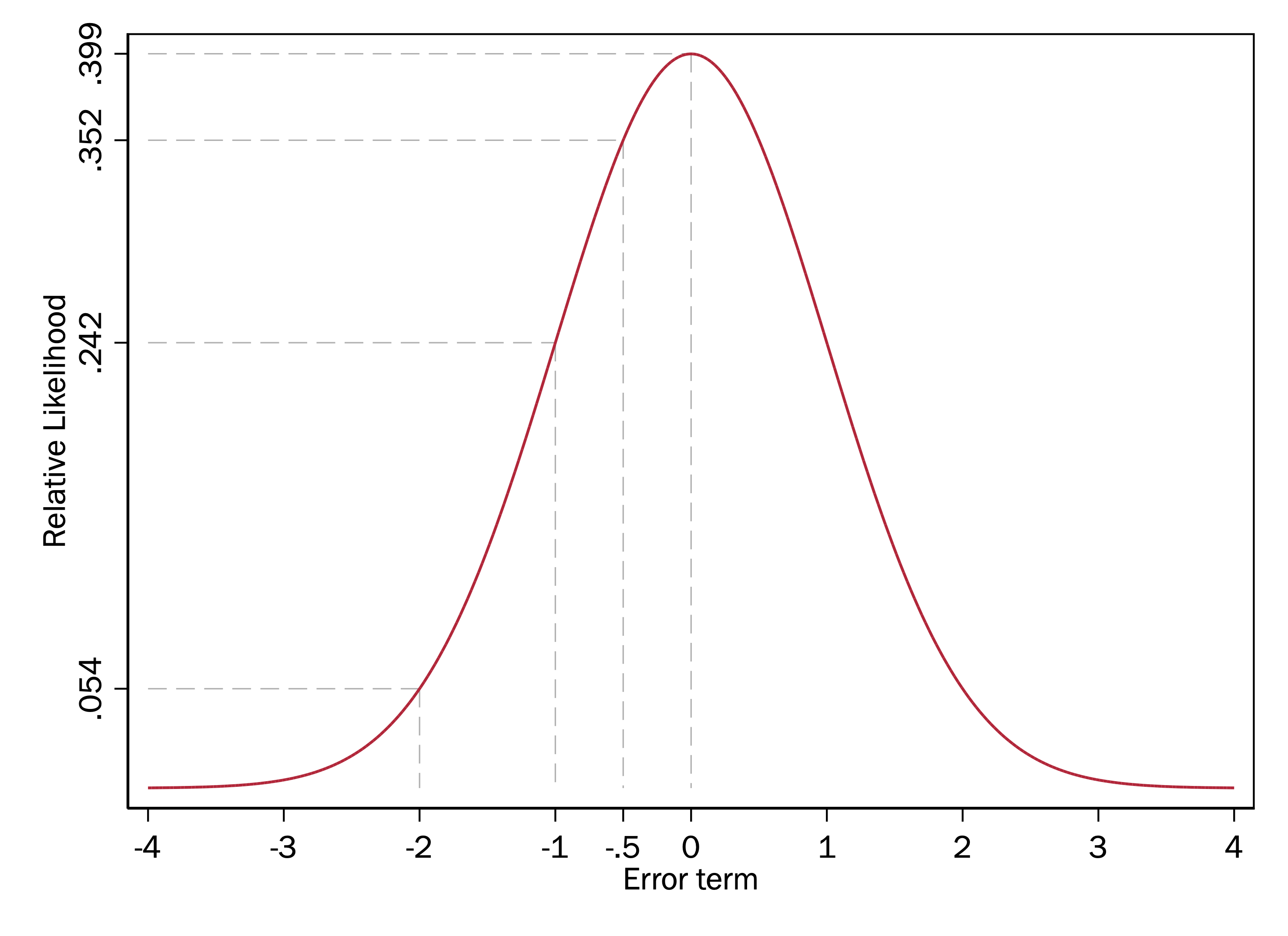
Now say we do indeed have a model in which the errors are normally distributed with a mean of zero and standard deviation of 1. Let’s redraw the standard normal above, highlighting some potential values of the error term:
If this is our error distribution, then, given that the highest point of the distribution is when \(x = 0\) (the mean), this graph indicates we are more likely to have an \(\varepsilon\) of 0 than any other value. The y-axis does not mean that the probability of the error term being 0 is .399–we will return to that later–but the heights of this normal curve do indicate the relative likelihood of observing an \(\varepsilon\) of one amount versus another.
In this example, the height (\(y\)-axis value) of the normal curve when \(x = 0\) is .399 and the height of the normal curve when \(x = -1\) is .242. Because .399/.242=1.65, this means that we are 1.65 times more likely to get a random draw of \(\varepsilon = 0\) than \(\varepsilon = -1\). Because the height of the normal curve at \(x = -2\) is .054 and .242/.054 is 4.48, we are 4.48 times more likely to get a random draw of \(\varepsilon = -1\) than \(\varepsilon = -2\).
Key points
- We can think of models like the linear regression model as having a systematic component (the \(\mathbf{x\beta}\)) and a stochastic component (the error).
- In the linear regression model, the error term is modeled as a independent random draw from a normal distribution
- The standard deviation of the error term in the linear regression model is the RMSE.
- The normal distribution can be used to tell us the relative likelihood of observing errors of different amounts, given our model.