Cumulative distribution function of the normal distribution
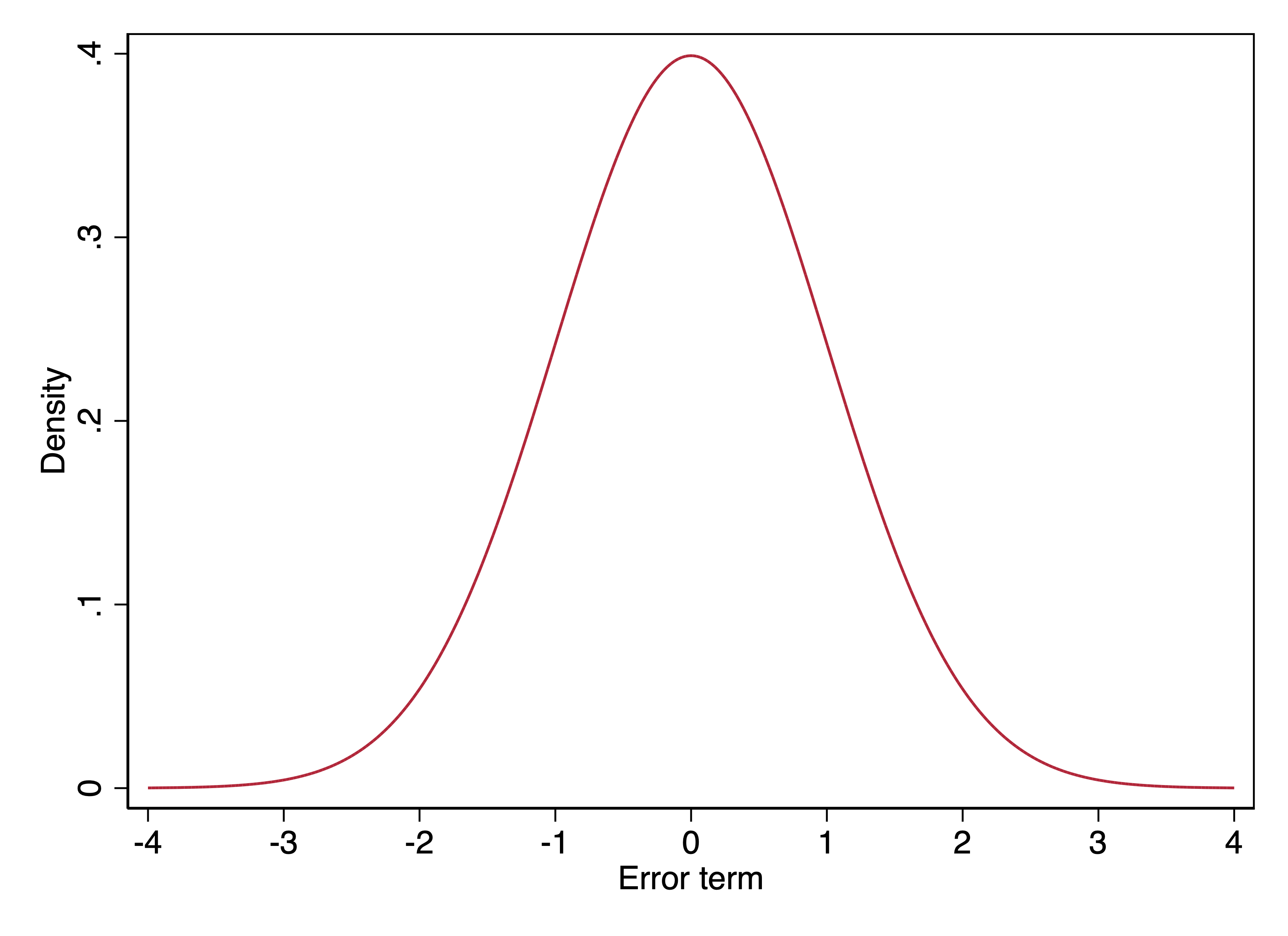
Above is the probability density function (PDF) of the standard normal distribution.
- What makes this the normal distribution is its shape.
- What makes this the standard normal distribution is the standard deviation is 1.
- What makes this a probability density function is that the area under the curve is 1 (that is, the total height \(\times\) width under the curve is 1).
Probability density functions represent probabilities in terms of the area under beneath the curve for different intervals along the horizontal axis.
For example, say the residuals in our statistical model was distributed as a standard normal. We could ask what the probability is that we would observe a value of a residual that is less than 0. This is the same as asking the area of the probability density function to the left of 0.
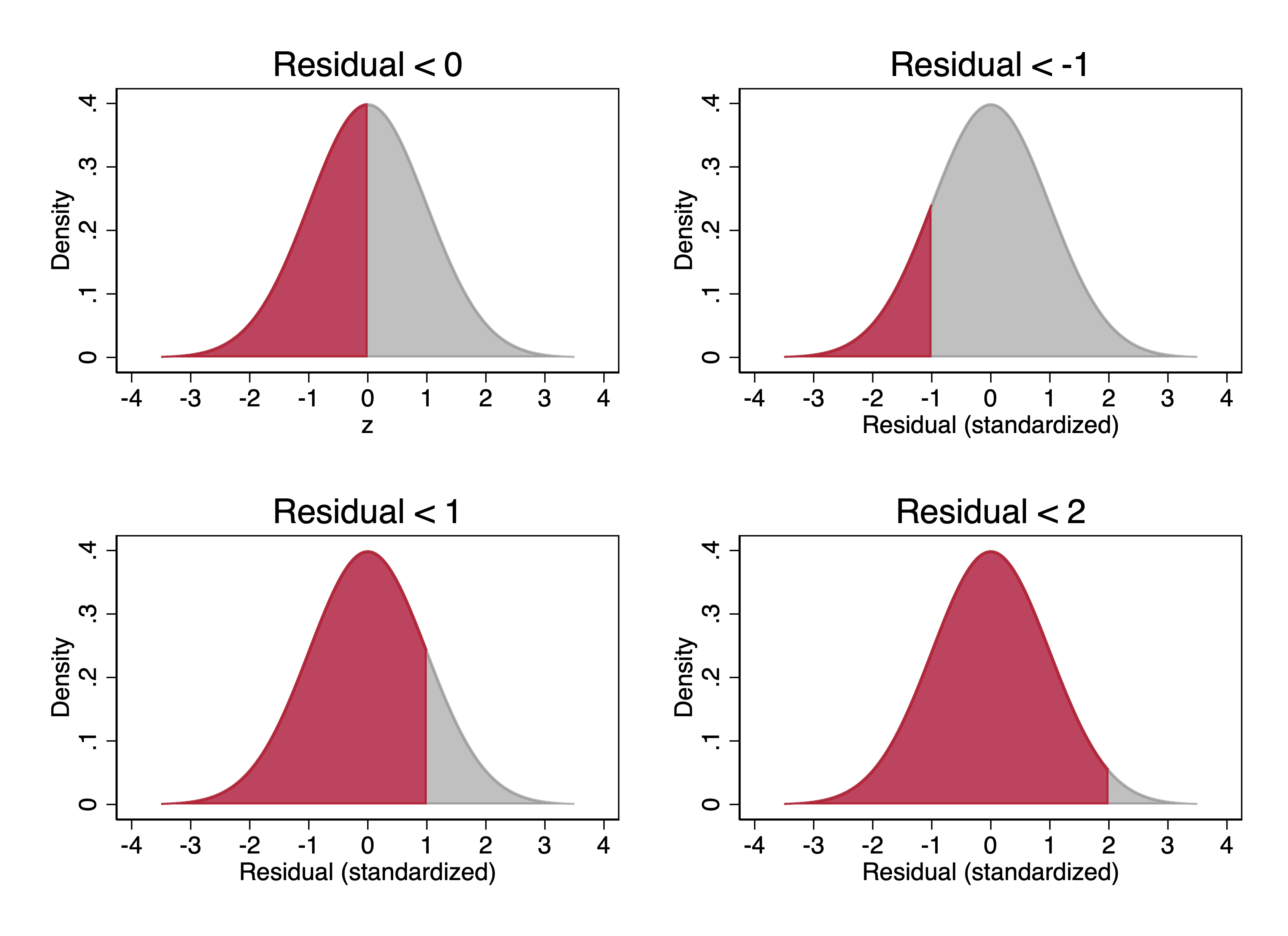
This is the area under the curve shown in red in the upper left graph above. Since it is half of the total area and the total area is 1, the area under the curve when the error is less than 0 is .5. This means that there’s a 50% chance that a random residual drawn from the standard normal distribution is < 0.
Instead of asking about the error being less than 0, we could ask about it being less than other values. The rest of the figure above shows the areas for an error less than -1, less than 1, and less than 2.
Stata: Normal PDF. In Stata, the function \(\texttt{normal()}\) provides the area to the left of \(z\) given the standard normal distribution.
. display normal(-1)
.15865525

. display normal(0)
.5

. display normal(1)
.84134475

. display normal(2)
.97724987
R: Normal PDF. In R, the function pnorm() provides the area to the left of \(z\) given the standard normal distribution.
> pnorm(-1)
[1] 0.1586553
For any value along the horizontal axis of \(z\), there is an area to the left of \(z\), and that is the probability of drawing a value \(< z\) at random from a standard normal distribution.
We can draw a graph that shows what this area under the curve for the standard normal distribution will be. This is known as the cumulative distribution function (CDF). Every PDF has a CDF: every probability density function has a corresponding cumulative distribution function.
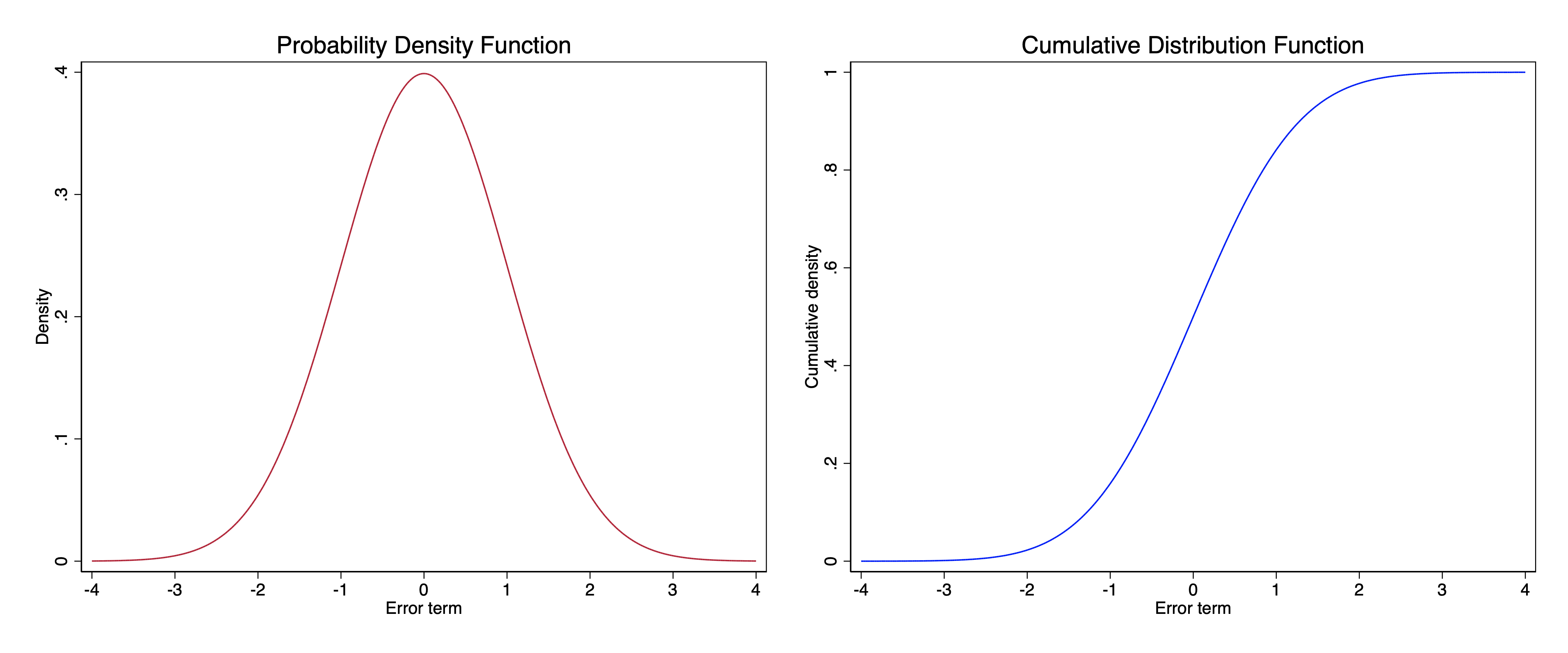
The graph above shows the probability density function and the cumulative distribution function for the standard normal distribution side-by-side.
Elaboration: If you’ve had some calculus: The cumulative distribution function is the integral of the probability density function, and the probability density function is the derivative of the cumulative distribution function.
Why is this important? We are about to connect two things:
- That the cumulative density function of the standard normal is a way of obtaining probabilities that involve the normal distribution.
- That the cumulative density function for the standard normal has a familiar shape. It is an S-curve. We have used a similar S-curve with the logit model for describing the relationship between the log odds of an outcome and the probability:
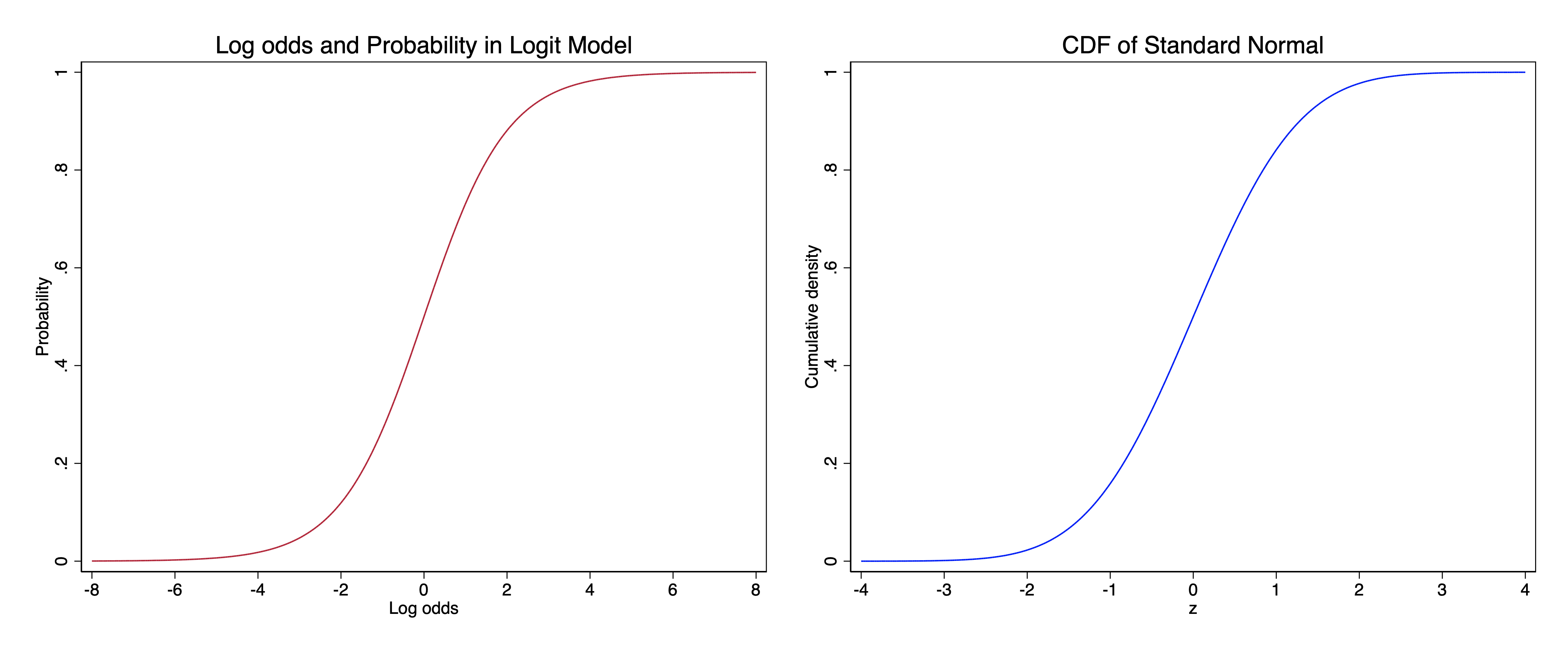
The S-curve on the left is the relationship between log odds and probability. The S-curve on the right is the relationship between a z-score and the cumulative density of the normal curve. Even just in terms of the curves themselves, they are not quite the same. For one thing, the horizontal axis values are different: the x-axis values in the logit model are more spread out. But even if we rescaled them, the curves wouldn’t exactly be the same; yet, as you can see, they look quite similar.
Part of our motivation for the logit model in the first place, compared to the linear probability model, is that we said that the S-curve provided a substantively realistic model in many cases for how we would expect changes in explanatory variables to affect probabilities. That is, we expect that often with binary outcomes, changes in explanatory variables will yield smaller changes in probabilities when the probabilities were near 0 or 1, and changes in an explanatory variable has the biggest effect when probabilities are around .5.
In the logit model, we obtain an S-curve by modeling a relationship that is linear in the log odds, because the relationship between log odds and probability is an S-curve. What we’ve just shown here, meanwhile, is that we can also easily get to an S-curve from the normal distribution: in that case, we just use its cumulative distribution function.