Testing for interaction via average change in probabilities
In 2018, the then-editors of American Sociological Review provided a “A Few Guidelines for Quantitative Submissions,” which included a statement about interactions in logit models:
“The case is closed: Don’t use the coefficient on the interaction term to draw conclusions about significance of statistical interaction in categorical models such as logit, probit, Poisson, and so on”
I disagree with their blanket conclusion that there is a problem with drawing conclusions from the statistical significance of the interaction term. And I am not alone!
But, this does represent a position that a fair number of folks hold, and therefore I will explain here what they recommend doing instead.
In Mize’s case, the argument runs like this. First, he argues that there is such a thing as a natural metric of an outcome variable:
“The goal of the analysis is to determine whether an interaction effect exists in terms of the natural measured metric of the dependent variable (for example, that the interest is in the effect on wages even when the log of wages is used as the dependent variable)”
And then he argues that, for logit/probit models, probabilities are the natural metric:
“in models such as binary, nominal, and ordinal logit/probit models… my assumption is that the metric of interest from these models is the predicted probabilities—not the odds, log odds, or latent variable metric”
From here, then, the conclusion is that the question as to whether there is an interaction effect is to be adjudicated in terms of whether there is a difference in terms of changes in probabilities.
Given the arguments for looking at the average predicted change (e.g., average marginal effect) as a way of talking in a summary way about a change in probabilities, the question of interaction then becomes a question of looking at differences in average marginal effects of those probabilities.
By this way of thinking, you can have a significant interaction even if the coefficient for the product term in your model is zero. To me, that is a problem with this way of thinking about interaction, at least substantively. But, to this other way of looking at it, the issue instead is with basing conclusions about interactions on the interaction term.
First differences after model with interaction term
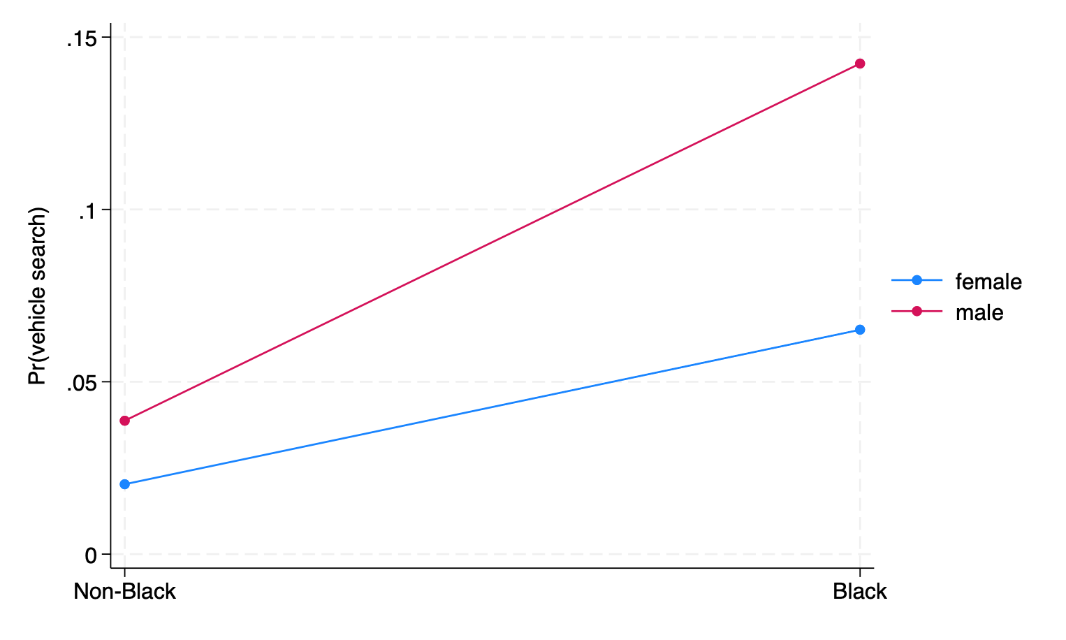
We will consider the example we were looking at earlier, from San Francisco traffic stops, and specifically the question of whether there is an interaction between Black (vs. non-Black) and sex on the probability of a vehicular search.
First, we fit a model with an interaction term between \(\texttt{male}\) and \(\texttt{black}\):
model <-glm(search_vehicle ~ male * black + tod + age + age_missing, data = df, family ="binomial")summary(model)
Call:
glm(formula = search_vehicle ~ male * black + tod + age + age_missing,
    family = "binomial", data = df)

Coefficients:
             Estimate Std. Error z value Pr(>|z|)
(Intercept) -2.989459   0.034023 -87.865  < 2e-16 ***
male         0.670572   0.021080  31.810  < 2e-16 ***
black        1.226056   0.032288  37.973  < 2e-16 ***
tod12am-3am  0.750063   0.028014  26.775  < 2e-16 ***
tod3am-6am   0.761389   0.040437  18.829  < 2e-16 ***
tod6am-9am  -0.070524   0.035013  -2.014    0.044 *
tod12pm-3pm  0.324746   0.027083  11.991  < 2e-16 ***
tod3pm-6pm   0.418641   0.026053  16.069  < 2e-16 ***
tod6pm-9pm   0.484914   0.026413  18.359  < 2e-16 ***
tod9pm-12am  0.557766   0.025728  21.680  < 2e-16 ***
age         -0.035345   0.000584 -60.521  < 2e-16 ***
age_missing -0.180279   0.029526  -6.106 1.02e-09 ***
male:black   0.219016   0.035615   6.150 7.77e-10 ***
---
Signif. codes:  0 '***' 0.001 '**' 0.01 '*' 0.05 '.' 0.1 ' ' 1

(Dispersion parameter for binomial family taken to be 1)

    Null deviance: 210032  on 563088  degrees of freedom
Residual deviance: 190633  on 563076  degrees of freedom
AIC: 190659

Number of Fisher Scoring iterations: 6
We can see that we have a significant interaction term for male:black (the last coefficient in the results).
. logit search_vehicle i.male##i.black ib4.timeofday age i.age_missing, allbaselevels

[output omitted]
Then we calculate the “first differences,” which in this case are the differences between men drivers who are Black vs. not-Black and the differences for women drivers who are Black vs. not-Black.
library(marginaleffects)mfx <-avg_comparisons( model,variables ="black", by ="male", comparison ="difference")mfx
 male Estimate Std. Error    z Pr(>|z|)     S  2.5 % 97.5 %
    0   0.0442    0.00158 27.9   <0.001 566.3 0.0411 0.0473
    1   0.1042    0.00149 70.0   <0.001   Inf 0.1012 0.1071

Term: black
Type: response
Comparison: 1 - 0
The difference between Black and not-Black men is 10.4 percentage points, while the difference between Black and not-Black women is 4.4 percentage points.
In Stata, we do this with the \(\texttt{margins}\) command.
. margins male, dydx(black) post

Average marginal effects                               Number of obs = 563,089
Model VCE: OIM

Expression: Pr(search_vehicle), predict()
dy/dx wrt:  1.black

------------------------------------------------------------------------------
             |            Delta-method
             |      dy/dx   std. err.      z    P>|z|     [95% conf. interval]
-------------+----------------------------------------------------------------
0.black      |  (base outcome)
-------------+----------------------------------------------------------------
1.black      |
        male |
     female  |   .0448473   .0016064    27.92   0.000     .0416989    .0479958
       male  |   .1036253   .0014839    69.83   0.000      .100717    .1065337
------------------------------------------------------------------------------
Note: dy/dx for factor levels is the discrete change from the base level.
In Stata, the option \(\texttt{post}\) for \(\texttt{margins}\) tells Stata to store the results from \(\texttt{margins}\) as estimation results. That is, the \(\texttt{logit}\) estimation results in memory are replaced by \(\texttt{margins}\) results, and we can do post-estimation operations on them.
Testing the second difference
In our case, we now want to test whether the difference between our two “first differences” – called the “second difference” is 0. This is the same as testing the equality of the two first differences.
In R, the marginaleffects package allows one to do this with its hypothesis argument. If you look at the output above, the difference we are trying to test is between the first and second row of the results. When we specify the hypothesis argument, we say to test that b2 = b1, which is that the estimate that would be in the second b2 and first row b1 of the usual avg_comparisons output are equal.
library(marginaleffects)mfx <-avg_comparisons( model,variables ="black", by ="male", hypothesis ="b2 = b1")mfx
The result can be interpreted as: - The male-female difference in the probability of a vehicle stop is 6 percentage points larger for drivers who are Black than drivers who are not Black (p > .001).
We can obtain the difference and a significance test for it using the \(\texttt{lincom}\) command:
. ** test of second differences using lincom
. lincom [1.black]1.male - [1.black]0.male

 ( 1)  - [1.black]0bn.male + [1.black]1.male = 0

------------------------------------------------------------------------------
             | Coefficient  Std. err.      z    P>|z|     [95% conf. interval]
-------------+----------------------------------------------------------------
         (1) |    .058778   .0021812    26.95   0.000      .054503    .0630531
------------------------------------------------------------------------------
The add-on Stata command \(\texttt{mlincom}\), which is part of the \(\texttt{spost13\_ado}\) package co-authored by yours truly, will do this with simpler syntax:
. ** test of second differences using mlincom
. mlincom 2-1

             |   lincom    pvalue        ll        ul
-------------+---------------------------------------
           1 |    0.059     0.000     0.055     0.063
The result can be interpreted as: - The male-female difference in the probability of a vehicle stop is 5.9 percentage points larger for drivers who are Black than drivers who are not Black (p > .001).
In the graph below, the first differences correspond to the vertical gap between the points for both non-Black and Black people. The question of whether the second difference is zero is asking whether the gap differs between those two groups, that is, whether the lines in the plot are parallel.
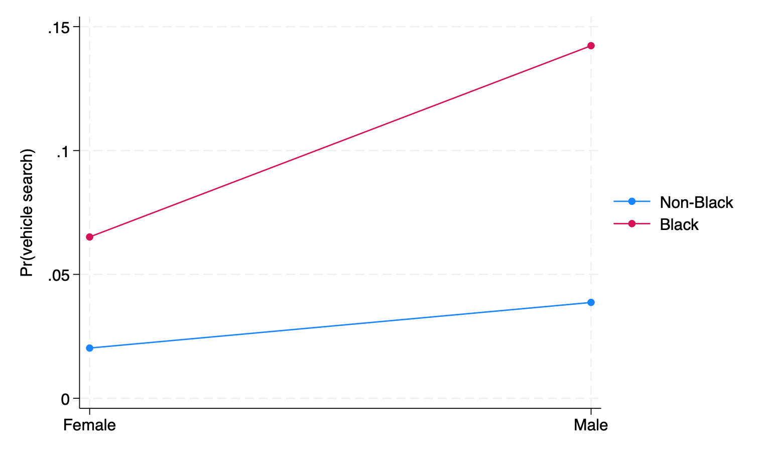
The first differences we computed above were the differences Black vs non-Black women and Black vs. non-Black men. But, we could have instead proceeded with the first differences being the comparisons between Black men vs. Black women and non-Black men vs. non-Black women. We would get different values for the first differences because we are calculating different quantities. But, in terms of the second differences, we would arrive at the same answer:
. quietly logit search_vehicle i.male##i.black ib4.timeofday age i.age_missing, allbaselevels

. margins black, dydx(male) post

Average marginal effects                               Number of obs = 563,089
Model VCE: OIM

Expression: Pr(search_vehicle), predict()
dy/dx wrt:  1.male

------------------------------------------------------------------------------
             |            Delta-method
             |      dy/dx   std. err.      z    P>|z|     [95% conf. interval]
-------------+----------------------------------------------------------------
0.male       |  (base outcome)
-------------+----------------------------------------------------------------
1.male       |
       black |
          0  |    .018429   .0005012    36.77   0.000     .0174467    .0194112
          1  |    .077207   .0021257    36.32   0.000     .0730407    .0813732
------------------------------------------------------------------------------
Note: dy/dx for factor levels is the discrete change from the base level.

. lincom [1.male]1.black - [1.male]0.black

 ( 1)  - [1.male]0bn.black + [1.male]1.black = 0

------------------------------------------------------------------------------
             | Coefficient  Std. err.      z    P>|z|     [95% conf. interval]
-------------+----------------------------------------------------------------
         (1) |    .058778   .0021812    26.95   0.000      .054503    .0630531
------------------------------------------------------------------------------
If we compare the plot below to the one above, you will see that the gap between lines in the plot below is larger. This is because the race gap in the probability of having one’s vehicle searched is larger than the sex gap.
Nevertheless, even though the gaps vary between the two plots, the extent to which the lines in each plot are non-parallel is the same in magnitude–this is the second difference.
Significant interactions without a significant interaction term
The idea with this understanding of statistical interaction is that the question of whether an interaction exists is not to be evaluated with reference to the interaction term, as the interaction term concerns log odds and the “natural metric” of the binary logit or probit model is probabilities.
While this approach implies that a significant interaction term in the model does not imply a significant interaction in the metric of probabilities, the converse is also true and more prominent in practice: the lack of a significant interaction term does not mean that there is not a significant interaction in terms of predicted probabilities.
One way to make sure the interaction term is zero is to omit it from the model entirely. When we do this for our example, we can see that we see that the second difference is still significant, although the estimate is different from before.
model_no_int_term <-glm(search_vehicle ~ male + black + tod + age + age_missing, data = df, family ="binomial")avg_comparisons( model_no_int_term,variables ="black", by ="male", hypothesis ="b2 = b1")
* no interaction term
. quietly logit search_vehicle i.male i.black ib4.timeofday age i.age_missing, ///
>         allbaselevels

. margins male, dydx(black) post

Average marginal effects                               Number of obs = 563,089
Model VCE: OIM

Expression: Pr(search_vehicle), predict()
dy/dx wrt:  1.black

------------------------------------------------------------------------------
             |            Delta-method
             |      dy/dx   std. err.      z    P>|z|     [95% conf. interval]
-------------+----------------------------------------------------------------
0.black      |  (base outcome)
-------------+----------------------------------------------------------------
1.black      |
        male |
     female  |   .0532362   .0009796    54.34   0.000     .0513162    .0551562
       male  |   .1000717   .0013535    73.94   0.000     .0974189    .1027245
------------------------------------------------------------------------------
Note: dy/dx for factor levels is the discrete change from the base level.

. lincom [1.black]1.male - [1.black]0.male

 ( 1)  - [1.black]0bn.male + [1.black]1.male = 0

------------------------------------------------------------------------------
             | Coefficient  Std. err.      z    P>|z|     [95% conf. interval]
-------------+----------------------------------------------------------------
         (1) |   .0468355   .0010912    42.92   0.000     .0446969    .0489742
------------------------------------------------------------------------------
The plot below contains the predictions here both in terms of log odds (left) and probabilities (right):
Because this is a logit model and there is no interaction term, we can see that the lines in the plot for log odds are parallel. The only way these lines could not be parallel is to fit a model that includes an interaction term. Nevertheless, if we look at the predicted probabilities, we can see that the lines are not parallel.
Indeed, if the baseline probabilities between two groups differ, then if the interaction term is zero, the second difference for predicted probabilities cannot be zero. So a model without an interaction term would in this case always show evidence of an interaction in terms of probabilities, as long as sample size is large enough.
As a result, then, in order for the test of whether there is an interaction in terms of probabilities to not be trivially true, we still need to include an interaction term. As odd as it sounds, perhaps, the interaction term is necessary to consider the possibility that there is not an interaction in terms of probabilities, which if baseline probabilities differ between groups can only happen if the interaction term in the model is itself non-zero.