Model dependence of statistical interactions for binary outcomes

A statistical interaction (aka interaction effect, aka moderation) occurs when the coefficient for one explanatory variable differs for different values of another explanatory variable.

Whether or not there is a statistical interaction is a often an especially model-dependent question, meaning that the answer may depend on how we have chosen to model the data. More bluntly, it is easy to overstate the extent to which statistical interactions reflect “reality” as opposed to “our model.”

This is a problem that lurks in linear regression. But, it is brought to the fore with binary outcomes.

We will provide two illustrations: one from our data on San Francisco traffic stops and one from our example of political donations by professors.

Simplest case: 2x2 interaction

In the traffic stop data, the outcome was whether a person who was stopped was subjected to a vehicular search. Black drivers were more likely than drivers who were not Black to have their vehicles searched, and men were more likely than women. Given these two findings, our result is whether there is also an interaction: are Black men even more likely to have their vehicles searched than we would expect given these two findings.

This is the simplest possible interaction, a 2x2 interaction between black/nonblack and male/female.

A longer way of wording the matter is whether, given the Black/non-Black difference among women and the male/female difference among non-Blacks, Black men are still more likely to have their vehicles searched. And, at least statistically, this is question is ultimately exactly the same as asking whether, given race and sex, non-Black women are even less likely than we would expect to have their cars searched, but we will present it here in terms of Black men.

What is the null hypothesis?

Let’s start by looking at the observed proportion of searches among vehicular stops for everyone but black men:

	Women	Men
Not Black	1.95%	3.83%
Black	7.27%	???

We can see there is a big difference among men and women among those who are not Black: 3.8% vs. 2.0%. And we can see there is an even bigger difference between being Black and non-Black among women: 7.3% vs. 2.0%.

Given these two differences, presumably any way we model the data would lead us to expect that, without a statistical interaction, the proportion of searches among stops for Black men is something higher than 7.3%.

But, how much higher? How much higher would we expect it to be if there wasn’t a statistical interaction?

After all, for the question of whether there is a statistical interaction to be sensible, there would have to be some proportion of searches that would lead us to conclude that there is not a statistical interaction. We would have to have, in effect, some sort of null hypothesis about what constitutes no interaction, and then we would consider whether what we actually observe is different from that.

The null hypothesis is model dependent

The null hypothesis depends on how we are modeling the data.

For the linear probability model, no interaction would imply that the difference in proportion between Black men and Black woman was equal to the difference in proportion between non-Black men and non-Black women. Because non-Black men are .0188 more likely to have their cars searched than non-Black women, the prediction for Black men if there was no interaction would be .0727 + .0188 = 9.2%.

We could instead fit a log-probability model, which is a model of the relative risk. Non-black men are 1.9 times more likely to have their cars searched than non-black women (3.83%/1.95% = 1.96). And thus, under this model, no interaction would mean we would expect the same for Black men compared to Black women. Since the proportion for Black women is 7.27%, the prediction for Black men would be \(7.27% x 1.96\) = 14.2%.

We have already shown how to calculate the relative risk from the odds ratio of the logit model, which in that case depends on the baseline probability. One can use Poisson regression to fit a log-probability model directly.

In the logit model, everything is converted to log odds. We start then by converting the observed proportions to log-odds: -3.223 for non-Black men, -3.918 for non-Black women, and -2.546 for Black women. The log odds for non-Black men is thus .694 more than the log odds for non-Black women. If there was the same difference for Black men compared to Black women, the log odds for Black men would be -1.852, for a predicted proportion of 13.6%

There is also the probit model, which involves us converting the observed proportions into “probits” using the inverse cumulative distribution function of the standard normal distribution: -1.771 for non-Black men, -2.064 for non-Black women, and -1.456 for Black women. The result is -1.163 for Black men, which we then convert back to a probability using the cumulative normal, which is 12.2%.

Four models, and four different answers as to what our null hypothesis of “no interaction” means. Just by choosing a different model, we can pick what we mean by no interaction from predictions for Black men.

Model	Prediction for Black men
Linear probability	9.2%
Probit	12.2%
Logit	13.6%
Log-probability	14.2%

As it happens, the actual proportion for Black men having their vehicle searched in these data is 15.6%. In our example, then, any of these ways leads to the conclusion that there is a positive statistical interaction: Black men are even more likely to get searched if stopped than what we would have expected.

But, imagine if we have observed a result close to 12.2%: depending on what model we were using, our interaction terms might have led us to conclude there was a positive interaction (linear probability), no interaction (probit), or a negative interaction (logit or log probability), and the fact that our conclusion depended on the model we chose might not have been apparent.

Categorical-by-continuous variable interaction

In the data on political contributions by professor, we found that men professors were more likely to donate to Republican presidential candidates than women, and that, the more Republican-leaning the congressional district in which a professor resides, the more likely they are to donate to a Republican (vs. Democratic) presidential candidate.

We can then ask whether there is an interaction: is the relationship between the red-ness of one’s congressional district and donating to a Republican candidate differ between men and women?

The table below shows results when we consider this question using both a linear probability model and a logit model. For each, we show estimates both with and without the interaction term.

options(scipen = 9)

library(tidyverse)
library(lmtest)
library(sandwich)

data <- read_csv("../csv/professor_contributions_2024.csv")

model_lpm <-   lm((rep_donor == "yes") ~ man + cpvi25_red, data = data)
coeftest(model_lpm, vcov=vcovHC(model_lpm)) # robust standard errors

model_lpm_int <-   lm((rep_donor == "yes") ~ man + cpvi25_red + (man*cpvi25_red), data = data)
coeftest(model_lpm_int, vcov=vcovHC(model_lpm_int)) # robust standard errors

model_logit <-   glm((rep_donor == "yes") ~ man + cpvi25_red, data = data, family="binomial")

model_logit_int <-   glm((rep_donor == "yes") ~ man + cpvi25_red + (man*cpvi25_red), data = data, family="binomial")

vcov_lpm <- vcovHC(model_lpm, type = "HC1")
vcov_lpm_int <- vcovHC(model_lpm_int, type = "HC1")

library(texreg)
screenreg(
  list(model_lpm, model_lpm_int, model_logit, model_logit_int),
    override.se = list(
    sqrt(diag(vcov_lpm)),
    sqrt(diag(vcov_lpm_int))
  ),
  override.pvalues = list(
    2 * pt(abs(coef(model_lpm)/sqrt(diag(vcov_lpm))), df = model_lpm$df.residual, lower.tail = FALSE),
    2 * pt(abs(coef(model_lpm_int)/sqrt(diag(vcov_lpm_int))), df = model_lpm_int$df.residual, lower.tail = FALSE)
  ),
  custom.model.names = c("LPM [1]", "LPM [2]", "Logit [1]", "Logit [2]"),
  custom.coef.map = list(
    "manyes" = "Man",
    "cpvi25_red" = "CPVI",
    "manyes:cpvi25_red" = "Man x CPVI"
  ),
  digits = 4,
  include.rsquared = FALSE,
  include.adjrs = FALSE,
  include.nobs = TRUE,
  include.loglik = FALSE,
  include.deviance = FALSE,
  include.aic = FALSE,
  include.bic = FALSE
)

==========================================================================
            LPM [1]         LPM [2]         Logit [1]       Logit [2]     
--------------------------------------------------------------------------
Man             0.0515 ***      0.0580 ***      0.9439 ***      0.9465 ***
               (0.0022)        (0.0024)        (0.0423)        (0.0425)   
CPVI            0.0017 ***      0.0013 ***      0.0313 ***      0.0390 ***
               (0.0001)        (0.0001)        (0.0013)        (0.0024)   
Man x CPVI                      0.0009 ***                     -0.0107 ***
                               (0.0001)                        (0.0028)   
--------------------------------------------------------------------------
Num. obs.   46510           46510           46510           46510         
==========================================================================
*** p < 0.001; ** p < 0.01; * p < 0.05

If we look at the results, we can see that the sign of the interaction term for Man x CPVI differs between the two models. From the linear probability results, the posiitve interaction term would indicate the the relationship between CPVI and donating to a Republican candidate is stronger for men. From the logit results, the negative interaction term would indicate that the relationship is stronger for women.

We can show this a different way. Instead of fitting linear probability model and logit models with an interaction term, we will fit separate models for men and women.

vcov_lpm_men <- vcovHC(lpm_men, type = "HC1")
vcov_lpm_women <- vcovHC(lpm_women, type = "HC1")

library(texreg)
screenreg(
  list(lpm_men, lpm_women, logit_men, logit_women),
  override.se = list(
    sqrt(diag(vcov_lpm_men)),
    sqrt(diag(vcov_lpm_women))
  ),
  override.pvalues = list(
    2 * pt(abs(coef(lpm_men)/sqrt(diag(vcov_lpm_men))), df = lpm_men$df.residual, lower.tail = FALSE),
    2 * pt(abs(coef(lpm_women)/sqrt(diag(vcov_lpm_women))), df = lpm_women$df.residual, lower.tail = FALSE)
  ),
  custom.model.names = c("LPM Men", "LPM Women", "Logit Men", "Logit Women"),
  custom.coef.map = list(
    "manyes" = "Man",
    "cpvi25_red" = "CPVI",
    "manyes:cpvi25_red" = "Man x CPVI"
  ),
  digits = 4,
  include.rsquared = FALSE,
  include.adjrs = FALSE,
  include.nobs = TRUE,
  include.loglik = FALSE,
  include.deviance = FALSE,
  include.aic = FALSE,
  include.bic = FALSE
)

=========================================================================
           LPM Men         LPM Women       Logit Men       Logit Women   
-------------------------------------------------------------------------
CPVI           0.0022 ***      0.0013 ***      0.0282 ***      0.0390 ***
              (0.0001)        (0.0001)        (0.0015)        (0.0024)   
-------------------------------------------------------------------------
Num. obs.  23567           22943           23567           22943         
=========================================================================
*** p < 0.001; ** p < 0.01; * p < 0.05

In the output above, you can see that the LPM coefficient for CPVI is bigger for men than for women (.0022 vs. 0013). But the logit coefficient for men is smaller than the logit coefficient for women (.0282 vs .0390).

Aside: The logit coefficients are much larger than the LPM in both cases, but this is due to the logit model measuring changes in the outcomes in log-odds and the LPM measuring them in probabilities.

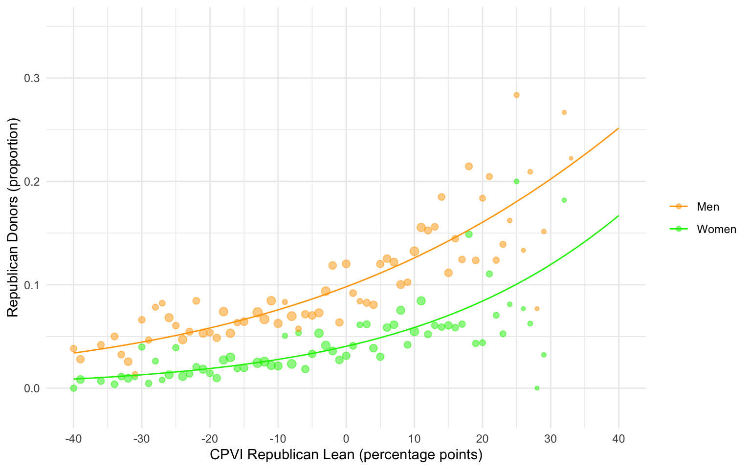
The reason for the difference might be clearer if we look at the data we are seeking to fit. Here is a plot of the proportion of Republican donors by each unique value of CPVI and by sex (using orange for men and green for women).

#| code-fold: true
#| code-summary: "Expand to see code to draw plot"
#| warning: false

plot_data <- data %>%
  filter(!is.na(man)) %>%
  group_by(cpvi25_red, man) %>%
  summarize(
    proportion_yes = mean(rep_donor == "yes", na.rm = TRUE),
    count = n()
  )

`summarise()` has regrouped the output.
ℹ Summaries were computed grouped by cpvi25_red and man.
ℹ Output is grouped by cpvi25_red.
ℹ Use `summarise(.groups = "drop_last")` to silence this message.
ℹ Use `summarise(.by = c(cpvi25_red, man))` for per-operation grouping
  (`?dplyr::dplyr_by`) instead.

plot <- ggplot(plot_data, aes(x = cpvi25_red, y = proportion_yes, color = man)) +
  geom_point(aes(size = count), alpha = .5) +
  scale_color_manual(
    values = c("yes" = "orange", "no" = "green2"), 
    labels = c("yes" = "Men", "no" = "Women"),
    name = NULL  # remove the legend title
  ) +
  scale_x_continuous(limits = c(-40, 40), breaks = seq(-40, 40, by = 10)) +
  scale_y_continuous(limits = c(-.02, .35)) +
  labs(
    x = "CPVI Republican Lean (percentage points)",
    y = "Republican Donors (proportion)"
  ) +
  theme_minimal() +
  guides(size = "none") 
plot

Warning: Removed 3 rows containing missing values or values outside the scale range
(`geom_point()`).

This plot shows that men have a consistently higher probability of being Republican donors and that, for both sexes, the proportion of Republican increases as the Republican lean of the professor’s congressional district increases.

Now let’s look at the same plot with the regression lines from the linear probability model added:

plot_lpm <- plot +
  geom_smooth(method = "lm", se = FALSE, linewidth = .5) 
plot_lpm

The regression line for men (orange) is steeper than the regression line for women (green). The difference in slopes is what is captured by the interaction term.

If we look closer, we can also see that the LPM misfits the data in a similar way to what we have elsewhere seen for lower-probability outcomes. Both regression lines are more likely to be higher than the actual proportions in the middle and lower on the ends. For women, the regression line dips below 0 on the y-axis, meaning that there are negative predicted probabilities for the women professors in the most Democratic leaning districts.

We can contrast this plot with the lines implied by the logit model:

pred_data <- expand.grid(
  cpvi25_red = seq(-40, 40, by = 1),
  man = c("yes", "no")
)

# Get predictions from the model
pred_data$predicted <- predict(model_logit_int, newdata = pred_data, type = "response")

plot_logit <- plot + 
    # Logistic curves
  geom_line(data = pred_data, 
            aes(x = cpvi25_red, y = predicted, color = man),
            linewidth = .5) 

plot_logit

For these logit curves, that the curve for women is steeper than the curve for men may be harder to see. If we look at the curve for men, we can see that the y-axis is about .05 when CPVI is -25, and it is about .1 when CPVI is 0. So, for men, the change from a 5% to 10% chance of being a Republican donor spans about a 25 point increase in CPVI.

If we look now to the logit curve for women, we can see that the y-axis is about .05 when CPVI is about 5, and then the y-axis is about .10 when CPVI is about 25. So, for women, the change from a 5% to 10% chance of being a Republican donor spans about a 20 point increase in CPVI. If we selected any point on the y-axis and slid the green curve for women to the left so that it overlapped with the orange curve for men, the green curve would be steeper than the orange curve. The corresponds to the logit coefficient for women being greater than the logit coefficient for men.

What to do?

The key takeaway here is that answering the question of whether there is a statistical interaction can depend on what “no interaction” means, and that in turn depends even in the simplest case on our choice of statistical models.

Often, when people want to talk about statistical interactions, they do so because they want to connect them to substantive claims: namely, that a significant interaction suggests a substantive difference in the outcome-generating process between the groups in question.

In that case, if one has chosen one’s model largely for arbitrary or convenience reasons, then typically, one does not want substantive conclusions to hinge on the choice.

A happy possibility, illustrated by our example of police stops, is that even when conclusions about interactions could differ by model, the pattern is sufficiently strong that it is robust. Seeing if this is so can involve fitting the model using different plausible specifications.

If the interaction does depend on the model choice, then for any substantive interpretation, it becomes pressing whether the model itself can be justified substantively. My own view would be that if one thinks, e.g., that the logit model provides the best characterization of how predictions about the outcome are related to the explanatory variable, then that would imply that this is also the substantive metric by which one should think about interactions.

All this, incidentally, refers to interactions that are sometimes called quantitative interactions. In our example, all of the models led to the expectation that the proportion of searches for Black men was greater than that for Black women, given that the proportion for non-Black men was greater than that for non-Black women. We were expecting the proportion to be more, and the question was how much more would we expect if there was no interaction. It would not be model-dependent, on the other hand, if Black men were actually less likely to be have their vehicles searched than Black women.