Probability is the most intuitive metric for thinking about the chance of something happening. While debates about exactly what probabilities are can get into the philosophical weeds quickly, we are going to stay pragmatic. Consider the notion that a set of meteorological conditions leads to a .30 probability of rain in the next 24 hours. We can take this as meaning that, if we observed a large number of different instances with those same meteorological conditions, it would rain in the next day 30% of the time, and the other 70% of the time it would not rain.
Aside: The idea that a 30% chance of rain means “if we observed a large number of different instances with those same meteorological conditions, it would rain in the next day 30% of the time” is an example of what is known as the frequentist interpretation of probability, for it interprets statements about probability as being statements about the frequency that something would happen in a large number of similar circumstances.
The main alternative to this view is the Bayesian interpretation of probability, in which probability statements reflect the strength of belief that an event will happen.
Probabilities are never less than 0 or greater than 1. This creates a problem for the linear probability model, because the predicted probability is the linear predictor, which is not constrained to values between 0 and 1.
That problem leads us to consider some alternative ways of talking about the chance of something happening. The first is the odds, and the second is the log odds, which is also known as the logit.
Odds
The odds of an event happening is the ratio of the probability of it happening to the probability of it not happening. That is:
To give an example, on the eve of the 2016 US presidential election, the (now-defunct) website fivethirtyeight forecast Donald Trump as having a .29 probability of winning, and Hillary Clinton as having a .71 chance. So, if this website was right, then Hillary Clinton’s odds of winning were:
Some particularly noteworthy examples of the relationship between probability and odds:
If the probability of an event is .5, then the odds are \(.5/.5 = 1.\)
If the probability of an event is nearly 1, then the odds are very large. For example, the odds when the probability is .999 are \(.999/.001 = 999\).
If the probability of an event is nearly 0, then the odds are very small, but odds are never negative. For example, the odds when the probability is .001 are \(.001/.999 = .001\).
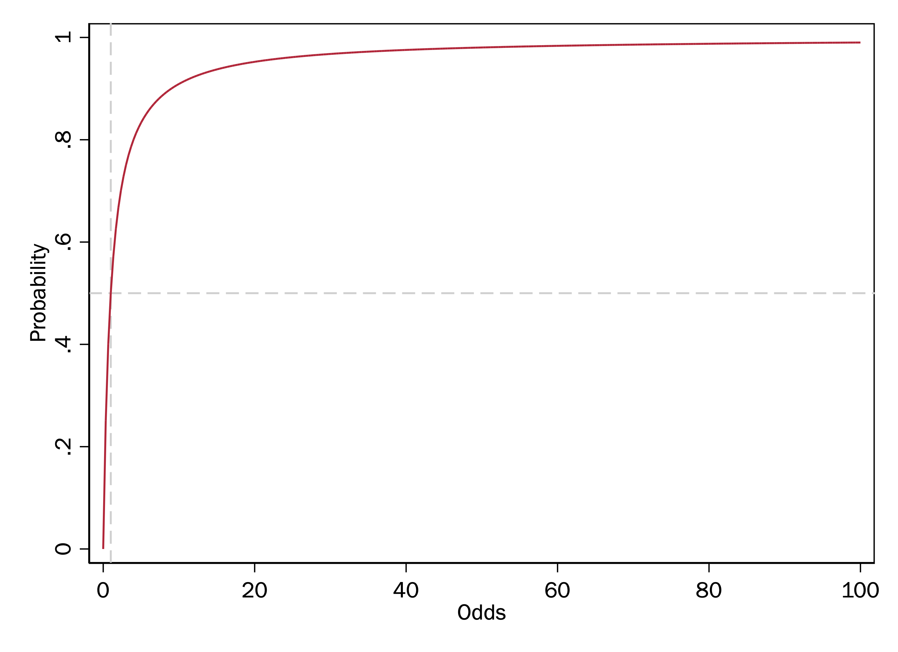
Remember: the problem that the linear predictor poses for the linear probability model is that probabilities are constrained between 0 and 1, whereas the linear predictor can range from \(-\infty\) to \(+\infty\). Odds only half-solve this problem. Even though the maximum possible odds are \(+\infty\), the minimum possible odds, like probabilities, are 0. We need a transformation that maps values between 0 and 1 onto a scale from \(-\infty\) to \(+\infty\).
A particularly enduring use of odds is for gambling. Say you were a bookie taking bets on the 2016 election. Since Hillary Clinton was more likely to win, a bet on Clinton should not have offered the same potential return as a bet on Trump. Odds provide the fair amount that somebody should have to wager in order to win $1 if their bet is correct.
That is, if the probabilities provided by fivethirtyeight were correct, someone wagering on Clinton should have had to pay $2.45 in order to win $1 had Clinton won, meaning that they would take home $3.45 ($1 plus getting their $2.45 back). In doing so, had Clinton won, they would have earned a 41% return on their bet, as \(\frac{1}{2.45} = .41\).
On the other hand, somebody betting on Trump would have only had to pay 41 cents (taking home $1.41). In doing so, they would have earned a 245% return on their bet, as \(\frac{1}{.41} \approx 2.45\).
Log odds (aka logit)
Any positive value can be logged. The range of possible log values is \((-\infty, \infty)\). Values greater than 1 will have a log value > 0, and values less than 1 will have a log value < 0. As a result, while odds only solved half our problem, logging the odds solves it entirely.
In our running example, the odds of a Hillary Clinton win in the 2016 election was 2.45, and the odds of a Donald Trump win was .41. We can convert these to log odds:
Elaboration: The logit of (y=1) and the logit of (y=0) are the same except for the sign. The reason this is the case is because the \(\textrm{odds}(y=1) \times \textrm{odds}(y=0) = 1\), and if \(a \times b = 1\), then \(\ln(a) + \ln(b) = \ln(1) = 0\), which in turn implies that \(\ln(a) = - \ln(b)\).
To convert log odds back to odds, we simply exponentiate the log odds (also called taking the antilog):
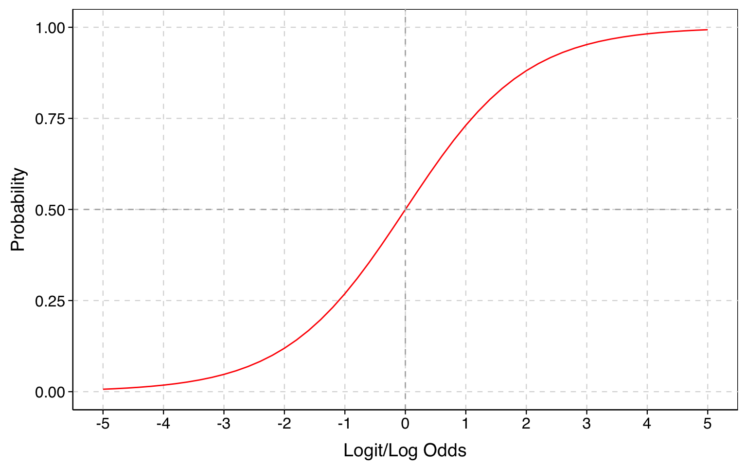
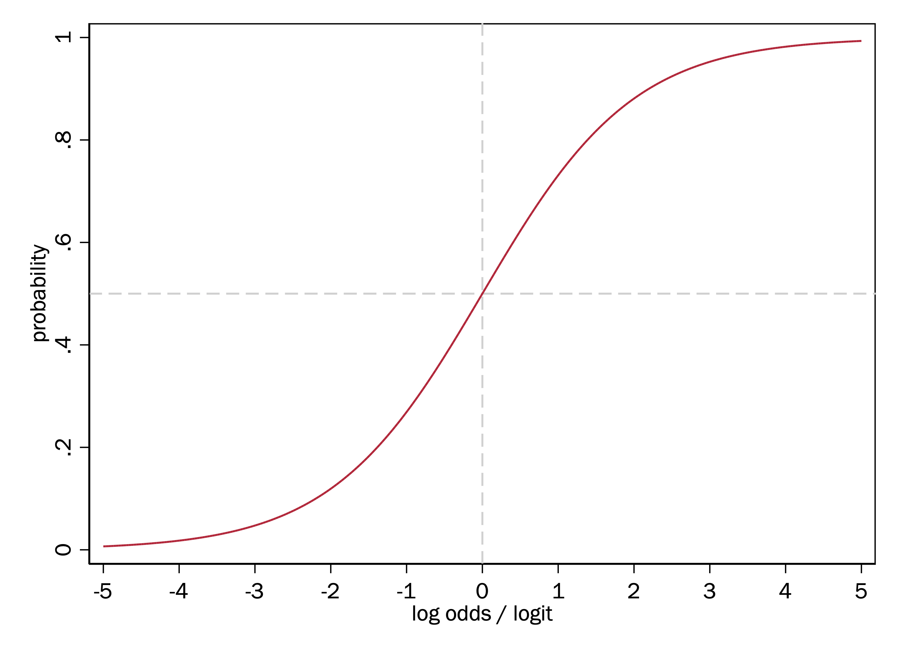
Take note of the S-shape of this function. This means a one-unit increase in log odds has different effects on the probability, depending on where on the x-axis we start. The effect is smallest for the most extreme values of log odds, and steepest in the middle.
This is substantively appealing because it reflects how we think probabilities may change in response to changes to many kinds of causal variables: where a given increase in a causal variable may have the biggest effect on the probability when the probability is intermediate, and has smaller effects when the probability is either very low or very high.
Functions with an S-shape like this are commonly referred to as sigmoid functions.
Summary of key points
Because probabilities are bounded by 0 and 1, a linear probability model can yield impossible predicted probabilities.
Probabilities are the most familiar way of thinking about the chance of something happening, but they are not the only way.
Odds transform a probability into \(\frac{p}{(1-p)}\). As a result, the range of odds is between 0 and infinity, with an odds of 1 meaning that an event has a probability of .5.
Log odds transform a probability into \(\ln\left(\frac{p}{(1-p)}\right)\). As a result, the potential range of log odds spans the entire range from negative infinity to positive infinity, with a log odds of 0 meaning an event has a probability of .5.
The log-odds function is also known as the logit function. The logit function has an S-curve (sigmoid) shape.
A model that is linear in the logit instead of linear in the probabilities will never produce impossible predictions, and reflects the intuition that bigger changes in an independent variable are needed to produce the same change in the predicted probability when the predicted probability is near 0 or 1.