The linear probability model (LPM) is the model implied by using standard OLS regression with a binary outcome variable.
There has been shifting wisdom about the linear probability model, especially in sociology. A short version of this history:
Some time ago, many social scientists would be simply taught that using the linear probability model was bad practice.
Nowadays, the model is viewed much more favorably, to the point of some considering it generally preferable to the usual alternatives.
Others think taking one’s enthusiasm that far is overblown.
As we will discuss – and as with so much in quantitative analysis – the best answer likely depends on one’s application.
As a purely signaling matter in social science, saying “linear probability model” has the virtue of indicating that you are aware that there are formal differences between the implied model and the familiar linear regression model for continuous outcomes, and that you are not simply using OLS because that is all you know.
Why the linear probability model is not the same as linear regression
The standard linear regression model for a single observation i is: \[
\begin{equation}
y_{i}=\mathbf{x}_{i}\mathbf{\beta }+\varepsilon _{i}
\end{equation}
\]
With a binary outcome, however, \(y_{i}\) can only take on two possible values:
\[
\begin{equation}
y_{i}=\left\{
\begin{array}{l}
1\text{ if }\unicode{x201C}\text{yes}\unicode{x201D} \\
0\text{ if }\unicode{x201C}\text{no}\unicode{x201D} %
\end{array}%
\right.
\end{equation}
\]
Think about what this means for \(\varepsilon_{i}\). For any value of \(\mathbf{x}\_{i}\mathbf{\beta }\), \(\varepsilon _{i}\) can only take on two possible values: 1. \(\varepsilon _{i}\) is \(-\mathbf{x}_{i}\mathbf{\beta }\) if \(y=0\), 1. \(\varepsilon _{i}\) is \(1-\mathbf{x}_{i}\mathbf{\beta }\) if \(y=1\).
Quick example: Say that \(\mathbf{x}_{i}\mathbf{\beta }\) was .63. Then, if the outcome was 0, the residual (\(\varepsilon _{i}\)) would be -.63 [because \(0-.63=-.63\)].
If instead the outcome was 1, the residual would be .37 [because \(1-.63=.37\)].
In the linear regression model, when we talk about what a coefficient \(\beta\) means, we will often appeal to the idea of how predictions about the outcome change as the explanatory variable changes. We might make a statement like:
Each additional inch of height is associated with an increase of .25 units in one’s predicted shoe size.
With a binary outcome, however, talking about a change in the predicted outcome per se doesn’t make any sense. The outcome is either 0 or 1. What changes is not the predicted value of outcome itself, but the predicted probability of the outcome being either 0 or 1.
In my experience, students find it very intuitive that, when we use OLS regression on a binary outcome, the resulting value of \(\mathbf{x}_{i}\mathbf{\beta }\) should be interpreted as a probability. If anything, the issue instead is that the interpretive step is so intuitive that students do not always notice it has been made.
But, let’s be clear that we have:
In the linear regression model, \(\mathbf{x}_{i}\mathbf{\beta } = \hat{y}_i\) , where \(\hat{y}_i\) is the predicted value of the outcome. This is the same as the estimated conditional mean of \(y\) among those who share the same values of explanatory variables \(\mathbf{x}_i\).
In the linear probability model, \(\mathbf{x}_{i}\mathbf{\beta } = \Pr(y_i = 1)\), or the predicted probability that \(y_i = 1\). This is the same as the estimated proportion of \(y = 1\) among those who share the same values of explanatory variables \(\mathbf{x}_i\).
We will write the linear probability model like this:
\[
\Pr(y=1|\mathbf{x}) = \mathbf{x}\mathbf{\beta }
\] where \(\mathbf{x}\) is a specific set of values of our explanatory variables.
Elaboration: Why doesn’t the linear probability model have an error term?
In the linear regression model, the error term captures the fact that actual values of \(y\) differ from the expected value of \(\mathbf{x}\mathbf{\beta}\). Under the standard assumptions, there is an expected distribution of \(y\) given many observations with the same \(\mathbf{x}\), where the expectation is the normal distribution with a standard deviation equal to the RMSE.
In the linear probability model, the binary outcome being a predicted probability provides the expected distribution of the outcome: for example, if the predicted probability is .7, the expectation is that 70% of the time we would observe \(y=1\), and 30% of the time we would observe \(y=0\). (The fact that predicted probabilities of a binary variable behave this way on their own constitutes an extremely simple statistical distribution, the Bernoulli distribution.)
Because probabilities in themselves provide for variation in the outcome among observations with the same \(\mathbf{x}\), there is no reason for an error term when we write the model.
Interpreting estimates from the linear probability model
A big appeal of the linear probability model is its ease of interpretation. For our example here, we will use General Social Survey data (through 2018), with the outcome being whether the respondent is a religious none–that is, somebody who responds “None” when asked for their religious affiliation.
First, let’s look at a binary explanatory variable: whether the respondent was raised in a household without religion (this is the single largest predictor of identifying as a religious none in the GSS data).
In the Stata tabs, the \(\texttt{relig\_none}\) variable is \(\texttt{norelig}\) and the \(\texttt{raised\_as\_none}\) variable is \(\texttt{norelig16}\).
Click for code that loads packages, load data, and does some preparatory coding
# install these packages if not already installedlibrary(tidyverse)library(lmtest)library(sandwich)library(haven)library(tulaverse)options(scipen =9)# read datasetgss <-read_dta("../dta/gss_norelig_thru2018.dta")# drop cases in cohort < 1900gss <- gss %>%filter(cohort >=1900|is.na(cohort)) %>%drop_na(norelig) %>%mutate(relig_none = norelig,raised_as_none = norelig16)
# linear probability model with binary explanatory variablemodel <-lm(relig_none ~ raised_as_none, data=gss, weights=(wtssall))tula(model, robust =TRUE)
# coeftest(model, vcov=vcovHC(model)) # other way to get robust standard errors
. regress norelig norelig16 [pweight=wtssall]
(sum of wgt is 60,849.1620679662)

Linear regression                               Number of obs     =     60,712
                                                F(1, 60710)       =    2312.23
                                                Prob > F          =     0.0000
                                                R-squared         =     0.1049
                                                Root MSE          =     .30812

------------------------------------------------------------------------------
             |               Robust
     norelig |      Coef.   Std. Err.      t    P>|t|     [95% Conf. Interval]
-------------+----------------------------------------------------------------
   norelig16 |   .4602375   .0095712    48.09   0.000     .4414779    .4789971
       _cons |   .0950164   .0013555    70.10   0.000     .0923596    .0976732
------------------------------------------------------------------------------
Results here use robust standard errors. In R, we can robust standard errors with the coeftest() function, which requires the lmtest and sandwich packages. When showing model results with tula(), we can obtain robust standard errors if we specify robust = TRUE. In Stata, robust standard errors are automatically invoked when one fits a model with weights.
Here are some equivalent ways to interpret this result:
Respondents who were not religious at age 16 are 46 percentage points more likely to identify as religious nones.
Being raised in a non-religious household is associated with an increase of .46 in the predicted probability of being a religious none as an adult.
The proportion of religious nones among those raised without a religious affiliation is .46 higher than the proportion of religious nones among those who were raised with a religious affiliation.
Because this is a binary explanatory variable with no other covariates, we can verify the result by comparing the proportion of religious nones across the two groups.
tulatab(raised_as_none, data = gss, mean=relig_none)
Mean of Religious none?
──────────────────────────┼────────────────────
 Raised without religion? │       Mean        N
──────────────────────────┼────────────────────
 0 relig family           │  .09674042   57,308
 1 fam not relig          │       .551    3,404
──────────────────────────┼────────────────────
                    Total │       .122   63,858
. table norelig16 [pweight=wtssall], stat(mean norelig)

------------------------------------
                         |      Mean
-------------------------+----------
Raised without religion? |
  relig family           |  .0950164
  fam not relig          |  .555254
  Total                  |  .1206024
------------------------------------
We see from this output that 55.5% of those who were not raised with a religious affiliation grow up to be a religious none themselves. Meanwhile, only 9.5% of those who were raised with a religious affiliation grow up to be a religious none. This difference – 46.0 percentage points – matches the coefficient for \(\texttt{raised\_as\_none}\) above.
Percentage points versus percent
Above, we interpreted a result like this (emphasis added):
Respondents who were not religious at age 16 are 46 percentage points more likely to identify as religious nones.
We did not say:
Respondents who were not religious at age 16 are 46 percent more likely to identify as religious nones.
A percentage-point difference is the difference between one percent value and another, like how the increase from 10% to 56% is 46 percentage points (because \(56 - 10 = 46\)). A percent increase implies a multiplicative change: a 46 percent increase from 10% is not 56%, but rather \(10 \times 1.46 = 14.6%\).
Linear probability model coefficients can be interpreted as percentage point differences.
Next, let’s consider a situation in which we have a continuous explanatory variable: education measured in years.
# coeftest(model, vcov=vcovHC(model)) is another way to get robust standard errors
. regress norelig educ [pweight=wtssall]
(sum of wgt is 63,882.2272758198)

Linear regression                               Number of obs     =     63,736
                                                F(1, 63734)       =     365.43
                                                Prob > F          =     0.0000
                                                R-squared         =     0.0065
                                                Root MSE          =     .32437

------------------------------------------------------------------------------
             |               Robust
     norelig |      Coef.   Std. Err.      t    P>|t|     [95% Conf. Interval]
-------------+----------------------------------------------------------------
        educ |   .0084645   .0004428    19.12   0.000     .0075966    .0093324
       _cons |   .0112421   .0056258     2.00   0.046     .0002155    .0222687
------------------------------------------------------------------------------
We could interpret this coefficient as follows:
Each additional year of education is associated with a .008 increase in the predicted probability of being a religious none.
On average, the proportion of those who say they have no religious affiliation increases by .008 with each successive year of education.
An additional year of education is associated with a .8 percentage point increase in the predicted probability of reporting no religious affiliation.
Second example: Political contributions
As a second example, I will look at contributions by professors to either Democratic or Republican candidates in the 2024 Presidential race. I am using the public version of the Database on Ideology, Money, in Politics and Elections (DIME) data. Some points about how I have handled the data:
By “professors”, I mean people that either had the word “professor” listed within their occupation variable or said they were an “educator” but at a college or university in their employer variable.
The outcome is whether the professor is a donor to either a Republican or Democratic candidate. If someone donated to candidates in both parties – the most common such combination was Nikki Haley (Republican primary) and Kamala Harris (in the general election)– I went with the party that received the higher dollar amount.
As variables not included in this example, retired means the occupation had “retired” or “emerit*” somewhere in it. The adjunct variable means occupation had “adjunct”, “visiting”, or “part time” in it.
Click for code that loads data
data <-read_csv("../csv/professor_contributions_2024.csv")
If we look at the basic proportions for our outcome variable, we will see that the distribution is very lopsided. More than 94% of the professors in the data were Democratic donors.
tulatab(rep_donor, data=data)
────────────┼─────────────────────
  rep_donor │     Freq.    Percent
────────────┼─────────────────────
  no        │    56,797      94.39
  yes       │     3,376       5.61
────────────┼─────────────────────
      Total │    60,173     100.00
The data thus indicate that only a small proportion of the professors who made donations for the 2024 Presidential election did so on the Republican side.
Continuous explanatory variable
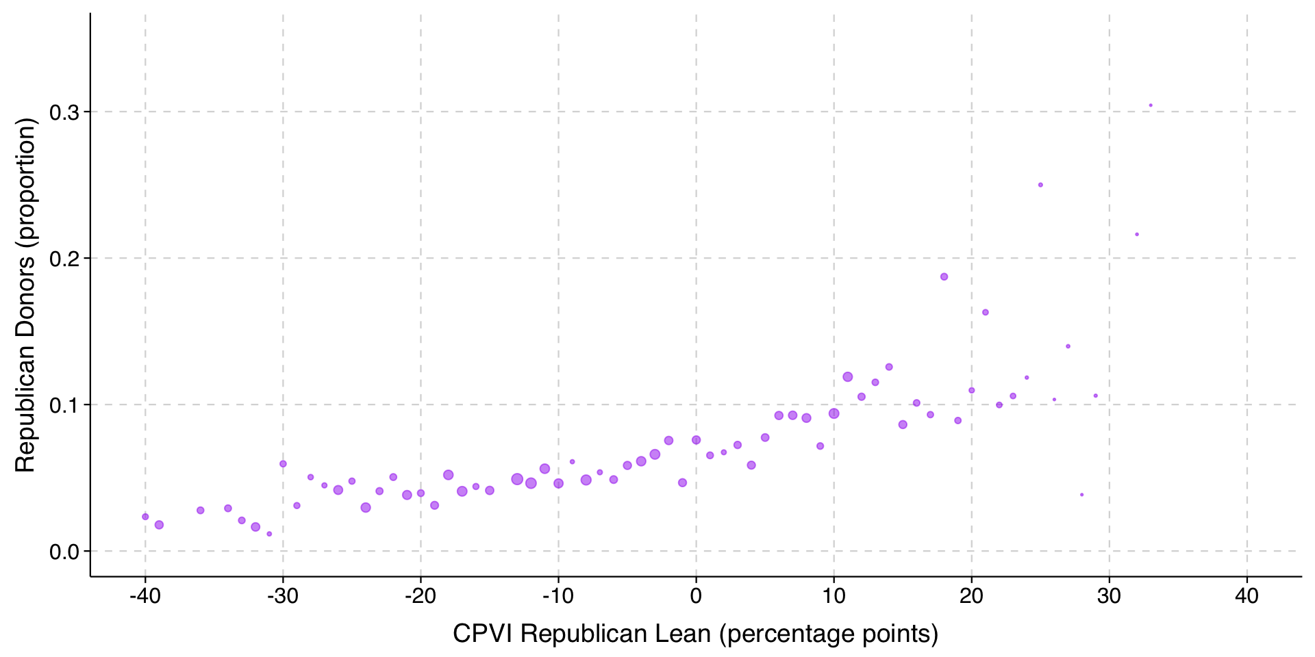
Is the proportion of Republican donors higher for professors in “red” regions of the country? The variable cpvi25_red is the Cook Partisan Voting Index (CPVI) at the congressional district level. It is coded so that 0 is a district with 0 lean toward either party, whereas each additional unit is a percentage point lean toward Republicans (so 5 is a Rep+5 district and -5 is a Dem+5 district).
The coefficient is .00175. We can interpret this as:
Among professors who donated to the 2024 Presidential election, a percentage point increase in the Republican lean of their congressional district is associated with a bit less than two-tenths of a percentage point increase in the proportion of Republican donors.
If we went from a very blue (-25 lean) to a very red (+25 lean), the expected proportion of Republican donors would increase by \(50\times(.00175) = .0875\), so nearly nine percentage points, a change that is all the more notable given the low proportion of Republican donors overall.
In this example, I will just talk about the probability of being a “Republican donor” rather than repeatedly saying a “Republican (vs. Democratic) donor.” But we are not talking about the probability of being a Republican donor for all professors, only those who donated to a major-party candidate.
Binary explanatory variable
Are professors at Ivy Plus universities who donate in Presidential Elections more or less likely to donate to Republican candidates? The variable ivyplus indicates whether a professor lists an Ivy Plus school as their employer.
ivyplus as used here includes the Ivy League schools plus Stanford, MIT, Northwestern, Chicago, Johns Hopkins, NYU, and Duke.
To see the bivariate relationship, we can compare the proportion of Republican donors across categories of ivyplus.
The positive coefficient of .046 for man == "yes" here can be interpreted as:
Net of being a professor at an Ivy Plus university, men professors are 4.6 percentage points more likely to be Republican donors than women professors.
The coefficient of ivyplus, on the other hand, did not change very much. Given that man is associated with the outcome, the lack of change in the ivyplus coefficient would suggest that ivyplus and man must have little or no association among professors who donated in 2024.
A variable we would expect to be associated with ivyplus is how Republican the professor’s congressional district is. After all, no Ivy Plus schools are located in especially red areas, and several are in famously Democratic strongholds. Let’s add cpvi25_red to the model:
model <-lm((rep_donor =="yes") ~ ivyplus + man + cpvi25_red, data = data)tula(model, robust=TRUE)
When we do this, the coefficient of ivyplus is diminished by over two-thirds of its magnitude in the previous model (from -.027 to -.008). This would indicate that being a professor at an Ivy Plus school is much less predictive of Republican donations once we account for the political lean of the surrounding area.
Impossible predictions
The 2025 CPVI has California’s 12th district (includes Berkeley) as the second-bluest district in the country, at D+39, or -39 points on the cpvi25_red variable in our model.
What is the predicted probability of a woman professor at UC-Berkeley donating to a Republican presidential candidate instead of a Democrat?
Using the coefficients above:
\[
\begin{align}
\Pr(y = \mathrm{Rep}) &= .0496 - (39 \times.00172) \\
&= .0496 - .0671 \\
&= -.0175
\end{align}
\] The predicted probability is -.0175, or an impossible value. Again, the linear probability model can yield predictions that are greater than 1 or (as in this case) less than 0.
Robust standard errors and the LPM
Throughout this page, we have used robust standard errors when fitting the linear probability model. Here is why.
The linear probability model is heteroskedastic by construction – meaning that the variance of the error term is not constant, but varies with \(\mathbf{x}\). This violates the OLS assumption of homoskedasticity (constant variance of the errors). As with non-normal errors, heteroskedasticity does not bias the coefficient estimates. But it does give us incorrect standard errors, which in turn means incorrect confidence intervals and incorrect \(p\)-values.
The reason the LPM is necessarily heteroskedastic is that the variance of a binary variable is entirely determined by its mean. If the mean of a binary variable is \(p\), its variance is \(p(1-p)\). In the LPM, the predicted probability \(\hat{y}|\mathbf{x}\) changes as \(\mathbf{x}\) changes; this is the whole point of the model. Since the variance of the error term is \(\hat{y}|\mathbf{x} \times (1-\hat{y}|\mathbf{x})\), it must also vary across observations. The heteroskedasticity is not incidental: it is a direct consequence of modeling a binary outcome.
Robust standard errors – also called heteroskedasticity-consistent standard errors – correct for this problem. Whenever we use the linear probability model, we should use them.
Robust standard errors differ by default in R and Stata.
If you compare estimates using robust standard errors in R and Stata, the estimates should match but the standard errors do not.
This is because there are several variants of the robust standard error, and R and Stata use different ones by default.
In R, if using coeftest() one can get the robust standard errors that Stata uses by adding the argument type = HC1. (With tula(), specify vcov="HC1") In Stata, the vce(hc3) option for estimation commands will use the robust standard errors that are the default in R.