Click for code that loads packages and data
library(tidyverse)
library(haven)
library(tulaverse)
gss <- read_dta("../dta/gss_norelig_thru2018.dta") %>%
    mutate(relig_none = norelig,
raised_as_none = norelig16)We wrote the linear probability model as:
\[ \Pr(y_i =1|\mathbf{x}_i)=\mathbf{x}_i\mathbf{\beta} \]
Similarly, we can write the logit model for binary outcomes as:
\[ \textrm{logit}(y_i=1|\mathbf{x}_i) = \ln\left[\frac{\Pr(y_i=1|\mathbf{x}_i)}{\Pr(y_i=0|\mathbf{x}_i)}\right]=\mathbf{x}_i\mathbf{\beta} \]
In this model, values of \(\hat{\beta}\) are coefficient estimates of the change in the logit of \((y=1|\mathbf{x})\).
Notice that \(\mathbf{x\hat{\beta}}\) is not \(\hat{y}\), demonstrating our earlier point that we need to refer to the linear predictor as \(\mathbf{x\hat{\beta}}\) because the linear predictor will not always be \(\hat{y}\).
Unlike the linear probability model, \(\mathbf{x\hat{\beta}}\) is not the predicted probability of \(y\). Instead, to obtain the predicted probability, we need to transform \(\mathbf{x\hat{\beta}}\).
\[ \widehat{\Pr}(y=1) = \frac{\exp(\mathbf{x}\hat{\mathbf{\beta}})}{\exp(\mathbf{x}\hat{\mathbf{\beta}}) + 1} \]
To illustrate, we use General Social Survey data on whether respondents report no religious affiliation, looking first at a categorical and then a continuous explanatory variable.
In these data (unweighted), we can first compare men and women on this outcome:
library(tidyverse)
library(haven)
library(tulaverse)
gss <- read_dta("../dta/gss_norelig_thru2018.dta") %>%
mutate(relig_none = norelig,
raised_as_none = norelig16)tulatab(male, data=gss, mean=relig_none, dec=3)Mean of Religious none?
──────────┼─────────────────
Male? │ Mean N
──────────┼─────────────────
0 female │ .094 36,050
1 male │ .155 28,475
──────────┼─────────────────
Total │ .121 64,525. table male, stat(mean norelig) nformat(%8.4f) nototal
------------------
| Mean
---------+--------
Male? |
female | 0.0938
male | 0.1551
------------------
Both of these proportions can be converted to log odds:
The log odds for men are \(-1.695 - (-2.268) = .573\) higher than for women.
When we fit the logit model with \(\texttt{relig\_none}\) as our outcome and \(\texttt{male}\) as our only explanatory variable, this difference of .573 is the coefficient we observe:
model1 <- glm(relig_none ~ male, data=gss, family="binomial")
tula(model1)
Family: binomial / Link: logit
AIC = 47010.951 Number of obs = 64525
BIC = 47029.101 McFadden R-sq = 0.01176
Log likelihood = -23503.476 Nagelkerke R-sq = 0.01655
─────────────────────────────────────────────────────────────────────────────
relig_none │ Coef Std. Err. z P>|z| [95% Conf Interval]
─────────────────────────────────────────────────────────────────────────────
male │ .5736 .02438 23.53 <.0001 .5258 .6214
(Intercept) │ -2.269 .01807 -125.6 <.0001 -2.304 -2.233
─────────────────────────────────────────────────────────────────────────────. logit norelig male
Iteration 0: log likelihood = -23783.213
Iteration 1: log likelihood = -23506.858
Iteration 2: log likelihood = -23503.476
Iteration 3: log likelihood = -23503.476
Logistic regression Number of obs = 64,525
LR chi2(1) = 559.47
Prob > chi2 = 0.0000
Log likelihood = -23503.476 Pseudo R2 = 0.0118
------------------------------------------------------------------------------
norelig | Coef. Std. Err. z P>|z| [95% Conf. Interval]
-------------+----------------------------------------------------------------
male | .5735747 .024381 23.53 0.000 .5257889 .6213605
_cons | -2.268581 .0180684 -125.56 0.000 -2.303995 -2.233168
------------------------------------------------------------------------------
We could write the results of the model as an equation, like so:
\[ \widehat{\textrm{logit}}(y_i=1) = -2.2685 + .5735(\texttt{male}_i) \]
For women, the estimated log odds are -2.2685, matching our calculation above.
For men, the estimated log odds are -2.2685 + .5735 = -1.6950, also matching our earlier calculation.
We can convert these log odds back to probabilities using the formula:
\[\widehat{\Pr}(y=1) = \frac{\exp(\textrm{logit}(y=1))}{\exp(\textrm{logit}(y=1))+1}\]
Taking men as our example, we convert this back to a probability:
\[ \hat{\Pr}(\mathrm{relig\_none}=1 | \mathrm{men}) = \frac{\exp(-1.6950)}{\exp(-1.6950) + 1} = \frac{.1836}{.1836 + 1} = .1551 \]
which matches the proportion of men reporting no religious affiliation shown above.
Now we will use respondent’s birth year as our explanatory variable. Here, we will look at the logit results first:
model2 <- glm(relig_none ~ cohort, data=gss, family="binomial")
tula(model2)
Family: binomial / Link: logit
AIC = 44444.177 Number of obs = 64319
BIC = 44462.320 McFadden R-sq = 0.0628
Log likelihood = -22220.089 Nagelkerke R-sq = 0.08675
─────────────────────────────────────────────────────────────────────────────
relig_none │ Coef Std. Err. z P>|z| [95% Conf Interval]
─────────────────────────────────────────────────────────────────────────────
cohort │ .03401 .0006659 51.07 <.0001 .0327 .03531
(Intercept) │ -68.44 1.305 -52.46 <.0001 -71 -65.89
─────────────────────────────────────────────────────────────────────────────. logit norelig cohort, nolog
Logistic regression Number of obs = 64,319
LR chi2(1) = 2977.93
Prob > chi2 = 0.0000
Log likelihood = -22220.089 Pseudo R2 = 0.0628
------------------------------------------------------------------------------
norelig | Coef. Std. Err. z P>|z| [95% Conf. Interval]
-------------+----------------------------------------------------------------
cohort | .0340069 .0006659 51.07 0.000 .0327018 .035312
_cons | -68.44223 1.304575 -52.46 0.000 -70.99915 -65.88531
------------------------------------------------------------------------------
Stata tip: Specifying the \(\texttt{nolog}\) option for \(\texttt{logit}\) and many other commands for fitting regression models suppresses the iteration log in the output, making it shorter.
We could write the model with our estimates as an equation:
\[ \mathrm{logit}(\texttt{relig\_none}=1) = -68.4423 + .0340(\texttt{cohort}) \]
So for someone born in 1940, our predicted log odds would be:
\[ \widehat{\mathrm{logit}}(\texttt{relig\_none}=1) = -68.4423 + .0340(1940) = -68.4423 + 65.9600 = -2.4823 \]
We could convert this back to a predicted probability as:
\[ \widehat{\Pr}(\texttt{relig\_none}=1) = \frac{\exp(-2.4823)}{(\exp(-2.4823) + 1)} = .077 \]
The logit model is linear in the logit, which means that a unit change in the explanatory variable is associated with a constant change \(\beta\) in the logit (log odds) of the outcome. That is, when the y-axis is log-odds, the fitted regression line is a straight line:
cohort = seq(1900, 1980, 2)
toplot <- data.frame(cohort)
toplot$pred_xb <- predict(model2, newdata=toplot)
toplot$pred_pr = exp(toplot$pred_xb) / (1 + exp(toplot$pred_xb))

# graph showing how model is linear in the logit
ggplot(data=toplot, aes(x = cohort)) +
    geom_line(aes(y=pred_xb), color="red3", linewidth=.75) +
    scale_y_continuous(breaks = c(-1, -2, -3, -4)) + expand_limits(y=c(-0.75, -4.25)) +
    scale_x_continuous(breaks = seq(1900, 1980, 10)) +
    theme_tula() +
    theme(panel.background = element_rect(fill = 'white', color = 'gray'),
          axis.text.x = element_text(size=10),
          axis.text.y = element_text(size=10)) +
    xlab("Year of birth") +
    ylab("Predicted log odds of outcome")

Our model predicts that each successive birth year will have the same increase in the log odds of having no religious affiliation, whether we are talking about successive birth cohorts in the 1920s or 1940s or 1970s.
While the logit model is linear, the transformation from log odds to probability is non-linear. As a result, the same plot with probabilities on the y-axis instead of log odds shows a non-linear curve:
ggplot(data=toplot, aes(x = cohort)) +
    geom_line(aes(y=pred_pr), color="red3", linewidth=.75) +
    scale_y_continuous(breaks = seq(0,  0.3, .05)) +
    scale_x_continuous(breaks = seq(1900, 1980, 10)) +
    theme_tula() +
    theme(panel.background = element_rect(fill = 'white', color = 'gray'),
          axis.text.x = element_text(size=10),
          axis.text.y = element_text(size=10)) +
    xlab("Year of birth") +
    ylab("Predicted probability of outcome")

Substantively, the increase between successive cohorts in the predicted proportion of respondents who identify as not religious is itself increasing with time.
The relationship between log odds and probabilities is an S-curve: while the probabilities always increase as log odds increase, the change is first very slow, then it accelerates until the change happens most rapidly when \(p=.5\), and then it decelerates and progressively slows as the probability approaches 1.
# relationship between probability and log odds

x <- seq(-5, 5, by=.2)
df <- data.frame(x)
df$y <- exp(df$x) / (1 + exp(df$x))

p <- ggplot(df, aes(x=x, y=y)) +
    geom_line(color="red3") +
    geom_hline(yintercept = .5, color="gray70", linetype="dashed") +
    geom_vline(xintercept = 0, color="gray70", linetype="dashed") +
    xlab("Logit/Log Odds") + ylab("Probability") +
    scale_x_continuous(breaks = seq(-5, 5, 1)) +
    scale_y_continuous(breaks = seq(0, 1, .2), limits = c(0, 1)) +
    theme_tula() +
    theme(panel.background = element_rect(fill = 'white', color = 'gray'),
          axis.text.x = element_text(size=10),
axis.text.y = element_text(size=10)) 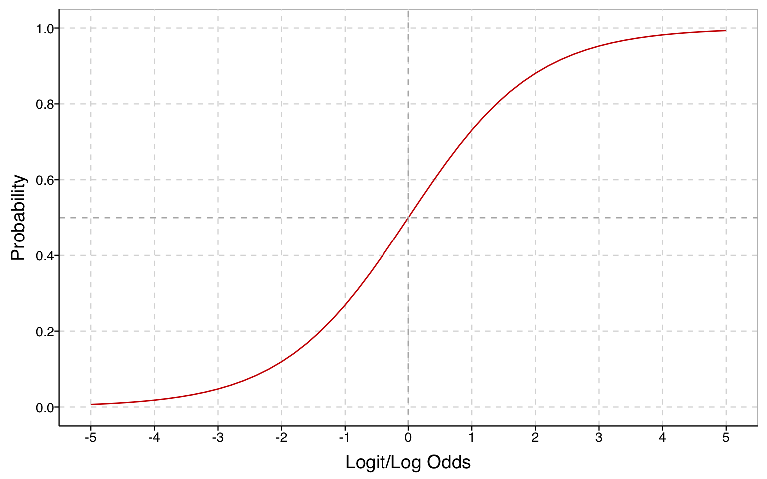

In the logit model, the right-hand side of the equation is as it was for the linear probability model, but the outcome is
\[\ln\left[\frac{\Pr(y_i=1|\mathbf{x}_i)}{\Pr(y_i=0|\mathbf{x}_i)}\right]\] that is, the log odds that \(y=1\), which is the same as saying the logit of \(y=1\).
\(\mathbf{x}\mathbf{\beta}\) is the log odds of \(y=1\). If instead we want the probability that \(y=1\), we can obtain this as:
\[ \widehat{\Pr}(y=1) = \frac{\exp(\mathbf{x}\hat{\mathbf{\beta}})}{\exp(\mathbf{x}\hat{\mathbf{\beta}}) + 1} \]