Are non-normal residuals a problem for the linear probability model?

Note to self on why this is no longer included: The point about always using robust standard errors was put with the linear probability model materials. This brings in a regular point about regression models not requiring normally distributed errors that one could make in the context of teaching linear regression, but digressive here.

Binary outcomes can only take on two values: 0 and 1. A distribution with only two possible values cannot be normally distributed.

The linear probability model involves using OLS with a binary outcome, and you may have heard that OLS makes some assumption regarding the normal distribution.

Is this a problem?

The normality assumption is about the residuals, not the unconditional outcome

First, we should clarify a misconception that people sometimes have, which is sometimes poeple think linear regression model involves an assumption that the outcome variable is normally distributed. Hooboy is this wrong.

The assumption, such that it is, is that the error term is normally distributed.

We can write the linear regression model as:

\[ y_i = \mathbf{x}_i\mathbf{\beta} + \mathbf{\varepsilon}_i \]

(Notice: We are not talking about the predicted outcome \(\hat{y}\) here. We are talking about the actual, observed value of our outcome \(y\).)

For observations that share the same values for all explanatory variables \(\mathbf{x}\), \(\mathbf{x}\mathbf{\beta}\) is a constant. So, according to the model, differences in \(y_i\) for observations that share the same value of \(\mathbf{x}\) are due to having different values of the error term.

As a result, if the errors are normally distributed, then conditional on \(\mathbf{x}\), the outcome variable is normally distributed.

But a variable being normally distributed conditional on \(\mathbf{x}\) does not necessarily imply the variable is unconditionally normally distributed. For example, say your outcome is height and you have a sample of mothers and their toddlers. The mothers’ heights may be normally distributed, and the toddler’s heights may be normally distributed. Yet if you were to put the two together, the combined distribution would not be normally distributed: instead there would be a hump for mothers and a hump for toddlers and a big gap in between.

Non-normal residuals do not bias OLS coefficient estimates

The fact that the OLS assumption, such that it is, is about the errors instead of about the outcome itself doesn’t resolve our worry about its potential mischief for the linear probability model. Because applying OLS to a binary outcome just as surely results in non-normal residuals.

Consider that, if we consider our estimate of \(\Pr(y=1)\) to be \(\hat{y}\), then no matter what our value of \(\hat{y}\) is at any particular point along \(\mathbf{x}\), a residual in the linear probability model can only take on one of two values: either it is \(1-\hat{y}\) (if \(y=1\)) or it is \(-\hat{y}\) (if \(y=0\)). Since the residuals for any value of \(\mathbf{x}\) can only take on one of two values, they cannot possibly be normally distributed and so the assumption of normally distributed errors is violated.

Even if the residuals are not normally distributed, however, OLS remains an unbiased estimator of the conditional mean.

In the sense of what is needed to avoid having biased coefficients, OLS does not involve an assumption about the shape of the distribution of the error term at all.

For avoiding biased coefficients, the key assumptions about the error term in regression are that the population mean of the error term is 0 (both unconditionally and conditional on \(\mathbf{x}\)) and that error term is uncorrelated with the explanatory variables.

The lack of normally distributed residuals in the linear probability model does not result in biased estimates.

The problem is with the standard errors, not the coefficients.

Alas, establishing that our coefficients remain unbiased despite non-normal residuals does not get us out of the woods. Because we typically want to have proper standard errors to go along with our estimates, and the assumption of normally distributed residuals does undergird the calculation of standard errors in OLS. Incorrect standard errors imply incorrect confidence intervals and incorrect p-values.

Part of the problem for standard errors goes away with non-small samples

The problems that non-normal residuals pose for standard errors are worse in small samples and worse the greater the deviation of the residuals from normality. Indeed, due to the Central Limit Theorem, the consequence of non-normal errors per se diminishes fairly quickly as sample size increases. This is related to how inferential statistics for OLS are officially calculated using the t-distribution rather than the normal distribution, but how, as sample size increases, the t-distribution becomes closer and closer to the normal distribution.

Even with a few hundred cases, non-normal residuals per se does not pose much of a problem for the correct estimation of standard errors.

So the fact that the linear probability model implies non-normal residuals is not itself much of a problem either for the coefficients or the standard errors.

Heteroskedasticity is the bigger issue, but has a solution

Unfortunately, there is a different assumption of OLS about the error term, which is that the variance of the error term is constant over \(\mathbf{x}\). This constant variance is known as homoskedasticity, and its violation is known as heteroskedasticity.

The linear probability model does not just imply non-normal errors, but it also implies heteroskedasticity.

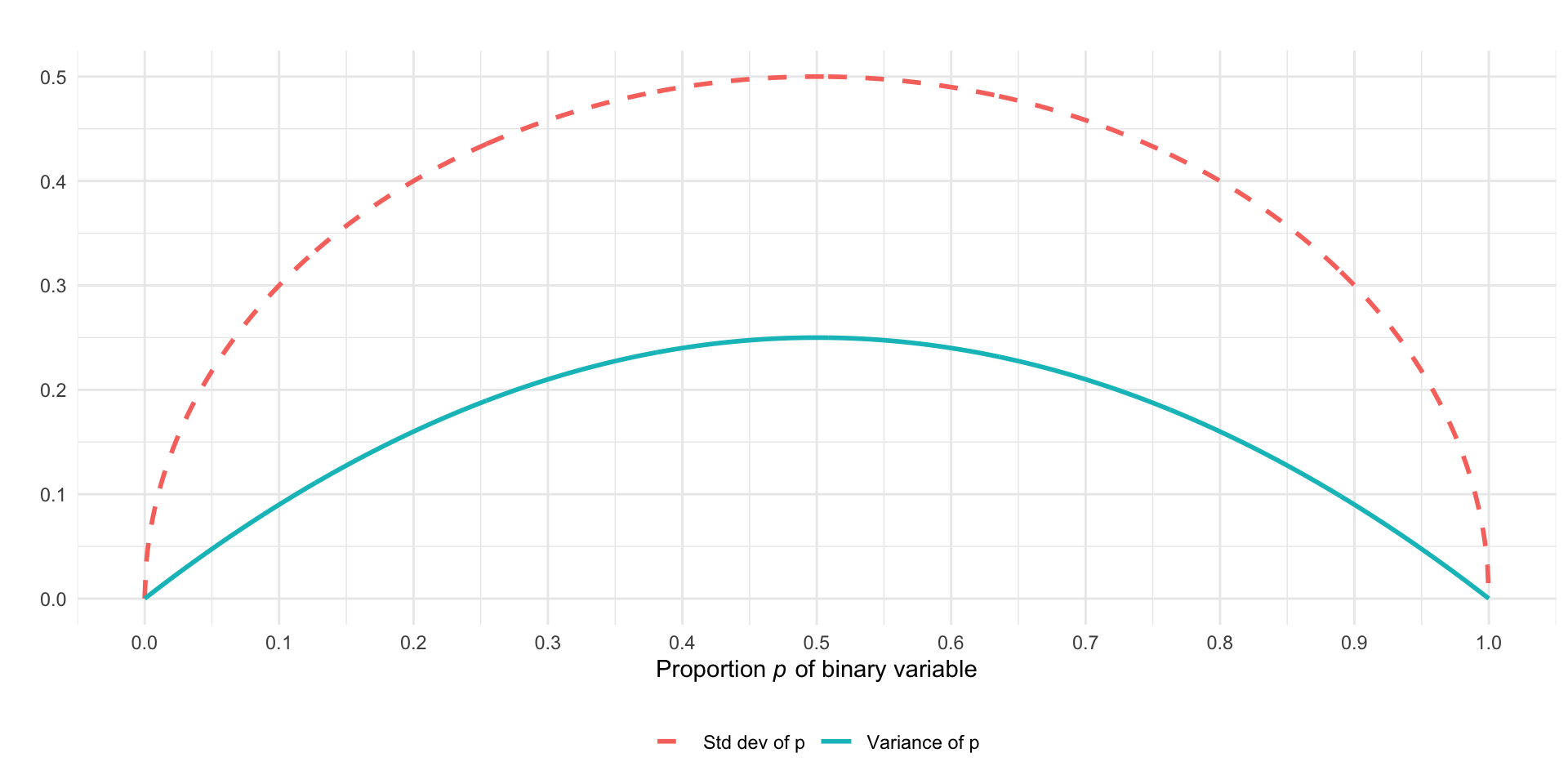
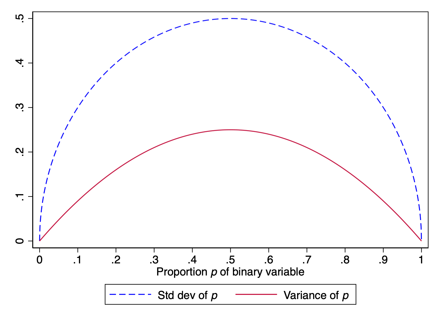
The reason why is that the variance of a binary variable is completely determined by its mean. Say the mean of a binary (0, 1) variable is \(p\). The variance is \(p(1-p)\).

#| echo: false

# Recreate the data in R
data <- data.frame(p = seq(0, 1, length.out = 1000)) %>%
  mutate(
    varp = p * (1 - p),
    sdp = sqrt(varp)
  )

# Create the ggplot
ggplot(data, aes(x = p)) +
  geom_line(aes(y = sdp, color = "Std dev of p"), linetype = "dashed", linewidth = 1) +
  geom_line(aes(y = varp, color = "Variance of p"), linewidth = 1) +
  scale_x_continuous(
    name = expression("Proportion " * italic("p") * " of binary variable"),
    breaks = seq(0, 1, 0.1)
  ) +
  scale_y_continuous(name = "") + # Remove default y-axis label
  theme_minimal() +
  theme(legend.position = "bottom", # Adjust legend position if needed
        legend.title = element_blank(), # Remove legend title
        axis.title.x = element_text(hjust = 0.5), # Center x-axis title
        plot.title = element_text(hjust = 0.5)) + # Center plot title if you add one
  labs(title = "") # Add a title here if desired

As a result, for a given \(\mathbf{x}\), the variance of the error term in the linear probability model is simply a function of \(\hat{y}|\mathbf{x}\). It is \(\hat{y}|\mathbf{x}\times(1-\hat{y}|\mathbf{x})\). Because \(\hat{y}|\mathbf{x}\) changes as \(\mathbf{x}\) changes, the variance of the error term must also change. Ergo, heteroskedasticity.

Again, violation of this assumption does not bias coefficients. OLS is a tough critter in this respect. But, as before, it has implications for the standard errors, and these implications are not so easily resolved by a larger sample size.

Nevertheless, we have a path forward. Robust standard errors are also known as heteroskedasticity-consistent standard errors because of their use to correct for heteroskedasticity.

Consequently, when we use the linear probability model, we should use robust standard errors.

Fitting the linear probability model with robust standard errors

In R, robust standard errors may be obtained using the \(\texttt{sandwich}\) package, commonly used in conjunction with the \(\texttt{lmtest}\) package. Unfortunately, there are at least seven subtly different types of robust standard errors, and the default that Stata uses and the default that the \(\texttt{sandwich}\) package uses are different. Stata’s default is “HC1” standard errors, while the \(\texttt{sandwich}\) package’s default is “HC3” standard errors (the “HC” stands for “heteroskedasticity consistent”).

# linear probability model with binary explanatory variable
model <- lm(relig_none ~ raised_as_none, data=gss, weights=(wtssall))
coeftest(model, vcov=vcovHC(model)) # robust standard errors


t test of coefficients:

                Estimate Std. Error t value  Pr(>|t|)    
(Intercept)    0.0950164  0.0013555  70.096 < 2.2e-16 ***
raised_as_none 0.4602375  0.0095753  48.065 < 2.2e-16 ***
---
Signif. codes:  0 '***' 0.001 '**' 0.01 '*' 0.05 '.' 0.1 ' ' 1

In Stata, one can obtain robust standard errors in Stata by specifying the option \(\texttt{robust}\) when fitting a regression model. If you want to obtain HC3 standard errors in Stata (i.e., those provided by default in R), specify the \(\texttt{vce(hc3)}\) option.

Summary of key points

To the extent OLS involves an assumption about normality, it is that the residuals are normally distributed, not the outcome itself.
- Normally distributed errors do imply the outcome is normally distributed conditional on the explanatory variables; in order words, normally distributed errors imply that a set of observations that share the same value of \(x\) are normally distributed.
As long as the mean of the errors is 0, OLS estimates are unbiased regardless of the shape of the distribution of the error function.
The residuals in the linear probability model are necessarily non-normal. However, this is not a problem for the estimates, and it is not a problem for the standard errors except in small samples.
The residuals in the linear probability model are necessarily heteroskedastic. This would be a problem for the standard errors in the linear probability model, but that problem can be addressed using robust standard errors.