Using the General Social Survey data on those who report having no religious affiliation, we can fit a logit model in which \(\texttt{male}\) and \(\texttt{cohort}\) are our explanatory variables.
# dependencies -- these packages need to be already installedlibrary(tidyverse)library(haven)library(tulaverse)options(scipen =9) # reduce amount of scientific notation in results# read datasetgss <-read_dta("../dta/gss_norelig_thru2018.dta") %>%mutate(relig_none = norelig,raised_as_none = norelig16)
model <-glm(relig_none ~ male + cohort, family="binomial", data=gss)tula(model)
Examples of how these logit coefficients can be interpreted are:
Net of birth year, the log odds of men reporting no religious affiliation are .57 higher than the log odds for women.
Holding sex constant, each successive birth cohort is associated with a .034 increase in the predicted log odds of reporting no religious affiliation.
The main problem with these interpretations is that a change in “log odds” is not a very meaningful metric to anyone not used to thinking in terms of logit coefficients.
One strategy for a more accessible interpretation of logit model results is to present results using odds ratios.
Explanation of the odds ratio using a 2x2 table
The 2x2 cross-tab below will help us understand what an odds ratio is. Our binary outcome provides the rows of the table and our binary explanatory variable provides the columns.
                │        Male?          │
Religious none? │    female        male │     Total
────────────────┼───────────────────────┼──────────
  Some religion │    32,670      24,058 │    56,728
                │     90.62       84.49 │     87.92
                │                       │
    No religion │     3,380       4,417 │     7,797
                │      9.38       15.51 │     12.08
────────────────┼───────────────────────┼──────────
          Total │    36,050      28,475 │    64,525
                │    100.00      100.00 │    100.00
. tabulate norelig male, col nokey

    Religious |         Male?
        none? |    female       male |     Total
--------------+----------------------+----------
Some religion |    32,670     24,058 |    56,728
              |     90.62      84.49 |     87.92
--------------+----------------------+----------
  No religion |     3,380      4,417 |     7,797
              |      9.38      15.51 |     12.08
--------------+----------------------+----------
        Total |    36,050     28,475 |    64,525
              |    100.00     100.00 |    100.00
Stata tip: By default Stata produces this “key” with the output to \(\texttt{tabulate}\) indicating what the cell values represent. You can turn this off with the option \(\texttt{nokey}\).
From the above, we can compute the odds of being a religious none separately for men and women:
The odds for men are: .1551/.8449 = .1835
The odds for women are: .0938/.9062 = .1035
Recall that odds are \(\Pr(y=1)/\Pr(y=0)\).
When we compare odds between groups, we do not take the difference. Instead, we use the ratio of the two odds. This is the odds ratio.
The odds ratio for men compared to women in this example is the odds for men divided by the odds for women. That is: .1835/.1035 = 1.773
If \(x\) is a binary variable, then the odds ratio is: \[\frac{\textrm{Odds}(x=1)}{\textrm{Odds}(x=0)}\]
In our example: \[\frac{\textrm{Odds}(\textrm{men})}{\textrm{Odds}(\textrm{women})}\]
Note that:
If the odds for men and odds for women were the same, the odds ratio would be 1.
If the odds for men are higher than the odds for women (as they are in this case), then the odds ratio for men vs. women will be greater than 1.
If the odds for women are higher than the odds for men, then the odds ratio for men vs. women will be less than 1.
But, because odds are always positive, odds ratios are always positive, so the odds would still be greater than 0.
With linear model coefficients, we are used to thinking about a positively signed coefficient as meaning an increase and a negatively signed coefficient as meaning a decrease. Instead, with odds ratios, an odds ratio above 1 means increasing odds and an odds ratio below 1 means decreasing odds.
Important:Odds and odds ratios are not the same thing. This is particularly confusing because the odds is defined as a fraction, \(\frac{\Pr(y=1)}{\Pr(y=0)}\), and so the odds is a ratio. But, the odds ratio is a ratio between two odds.
(If you think this is confusing, in the abstruse world of contingency table analysis there are also odds ratio ratios, which is the ratio between two odds ratios, so be thankful that at least you don’t have to keep that straight.)
Odds ratio for a binary explanatory variable
Let’s fit a logit model in which the outcome is \(\texttt{relig\_none}\) and the only explanatory variable is \(\texttt{male}\).
that is, the difference in the log odds for men vs. women. If we check, we can see that \(\ln(1.773) \approx .574\) (small difference due to rounding).
log(1.773)
[1] 0.572673
To get the odds ratio for men vs. women, we just take \(\exp(\beta_{male})\). More generally, the coefficients we estimate in our logit model can be interpreted as logged odds ratios. To get the actual odds ratio, we exponentiate the coefficient: \(\exp(\beta)\).
Odds ratio for a continuous explanatory variable
Now let’s look at the example of cohort as an explanatory variable using the same data.
The logit model is linear in the log odds. For continuous explanatory variable \(x\), the coefficient \(\beta_x\) in the logit model indicates the expected change in the log odds as \(x\) increases by one unit.
If we use \(c\) to indicate some particular value of \(x\), then \(\beta_x\) is the difference in the log odds when \(x=c+1\) vs. when \(x=c\).
\(\beta_x\) is the log of the odds ratio for a one-unit increase in \(x\).
Thus, if we take the exponent of \(\beta_x\), we get the odds ratio itself: \(\exp(.034) = 1.035\).
We can interpret this result as follows: as birth year increases by one unit, the predicted odds of not identifying as religious are 1.035 times the odds from the previous year.
Odds ratios are multiplicative changes: to get the odds after a multiplicative change, you multiply the odds before the change by the odds ratio. This is like how, if somebody gets a 10% raise, their new salary is 1.10 times their old salary.
Some general features of the odds ratio and the coefficients of the logit model:
If the odds ratio is 1, the odds will stay the same.
Also: If \(\exp(\beta_x) = 1\), then \(\beta_x = 0\)
If the odds ratio is greater than 1, the odds increase.
Also: If \(\exp(\beta_x) > 1\), then \(\beta_x > 0\)
If the odds ratio is less than 1, the odds decrease.
Also: If \(\exp(\beta_x) < 1\), then \(\beta_x < 0\)
Small coefficients provide approximation of odds ratio
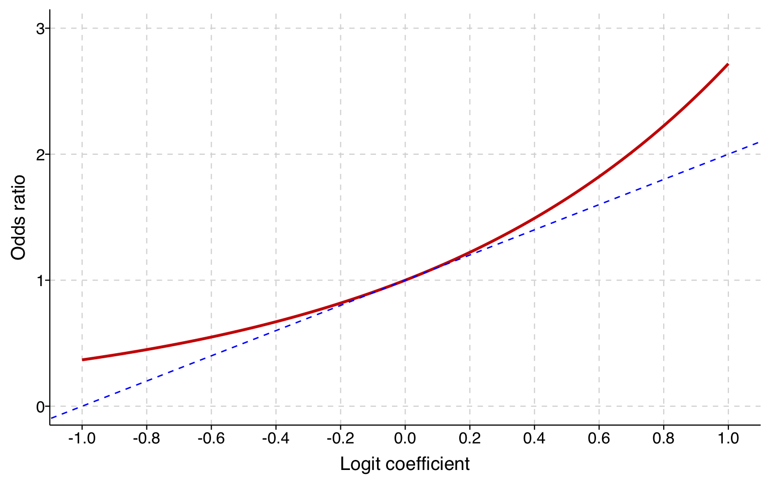
The closer a logit coefficient is to zero, the closer the odds ratio will be to \((1+\beta)\). For instance, in our example above, \(\beta\) for cohort was .034, and the odds ratio was 1.035.
The graph below shows the relationship between the odds ratio (\(\exp(\beta)\)) and \(\beta\). A dashed line is shown for reference at (\(\beta\), \(1+\beta\)). That the two lines are effectively on top of one another when \(\beta\) is between -0.1 and 0.1 shows that adding 1 to the logit coefficient is a very close approximation of the odds ratios when the coefficient is small. The approximation works less and less well as the magnitude of the coefficient increases.
Stata will exponentiate the coefficients for us if we include the \(\texttt{or}\) option for the \(\texttt{logit}\) command. Notice in the output below that the results are labeled “Odds Ratio.”
Stata: \(\texttt{logit}\) vs. \(\texttt{logistic}\). Stata has two commands that both fit the \(\texttt{logit}\) model: \(\texttt{logit}\) and \(\texttt{logistic}\). The difference is just in the output: by default, \(\texttt{logistic}\) provides odds ratios and \(\texttt{logit}\) provides coefficients. But, you can obtain odds ratios using the \(\texttt{logit}\) command with the \(\texttt{or}\) option. There is nothing wrong with using the \(\texttt{logistic}\) command, but personally for my own work I never do.
The odds ratio for male is 1.76. We can interpret this as:
Net of birth year and region of residence, the odds of identifying as non-religious are a factor of 1.76 higher for men than for women.
Net of birth year and region of residence, the odds of identifying as non-religious are 76% higher for men than for women.
For increases in the odds, we can talk about odds increasing by a factor of \(F\), or we can talk about the odds increasing by \((F-1)\times100\) percent.
We can interpret the odds ratio of 1.035 for cohort as:
Holding sex and region of residence constant, each successive birth year is associated with the odds of identifying as non-religious increasing by a factor of 1.035.
Holding sex and region of residence constant, each successive birth year is associated with a 3.5% increase in the odds of identifying as non-religious.
In the case of region, the reference category is living in the Northeast. The odds ratio of .626 for South can be interpreted as:
For those with the same sex and birth year, the odds of having no religious affiliation are lower for those in the South than for those in the Northeast by a factor of .63.
For those with the same sex and birth year, people living in the South have 37% lower predicted odds of not reporting a religious affiliation than people living in the Northeast.
For decreases in the odds, we can describe odds being lower by a factor of \(F\). In percentage terms, we talk about this change as being \((1-F)\times100\) percent lower.
Elaboration: Decreases in odds: Converting an odds ratio below 1 to a percentage change sometimes confuses people. An analogy: think about the price of goods that go on sale.
Say a store is having a sale on widgets and they are 20% off. A widget is normally $1.50. To figure out the sale price of the widget, you would multiply $1.50 by .8 ($1.20). In this example, the .8 is the factor change, and that it is less than one means the new price is lower than the original price. To get the percentage difference, we would subtract .8 from 1, getting .2, meaning 20% off.
Summary of key points
Logit model coefficients may be interpreted directly as changes in log odds, but this is not a very clear interpretation to many audiences.
If we exponentiate logit model coefficients, we get odds ratios, which can be interpreted as a factor change in the odds that y=1.
Factor changes may be easily converted to percentage changes. A factor change of 1.30 implies a 30% increase in odds, whereas a factor change of .70 implies a 30% decrease.