Expand for code that loads packages and data
library(tidyverse)
library(tulaverse)
library(marginaleffects)

data <- read_csv("../csv/professor_contributions_2024.csv") %>%
filter(!is.na(man))Relative risk, also called the risk ratio, refers to a multiplicative change in the probability of an outcome occurring.
That is, while the odds ratio provides interpretation in terms of a percent change in odds, relative risk refers to a percent change in the probability.
The advantage of relative risk is that it is more intuitive. The disadvantage is that, unlike the odds ratio, it depends on the baseline probability of the outcome; that is, it is not a quantity one can obtain just from the coefficient of the logit model.
In the data we have been looking at with campaign contributions, we will compute relative risk in the simplest case where we have only a binary explanatory variable (in this case, man).
library(tidyverse)
library(tulaverse)
library(marginaleffects)
data <- read_csv("../csv/professor_contributions_2024.csv") %>%
filter(!is.na(man))tulatab(man, mean=(rep_donor=="yes"), data=data)Mean of (rep_donor == "yes")
────────┼────────────────────
man │ Mean N
────────┼────────────────────
no │ .03231953 28,342
yes │ .07826665 28,569
────────┼────────────────────
Total │ .05538472 56,911The probabilities here are .0783 for men and .0323 for women. As we have no other explanatory variables to worry about, we can compute the relative risk easily:
\[ \frac{\Pr(\textrm{yes}|\textrm{man})}{\Pr(\textrm{yes}|\textrm{woman})} = \frac{.0783}{.0323} = 2.42 \]
This result may be interpreted as:
If we were interpreting this as a percent, 2.4 times as likely is the same as a 140% increase, not 240%. (Doubling an amount is increasing it by 100%.)
Notice there is no reference here to odds. Instead, we are talking about a ratio between two probabilities.
Using the avg_comparisons() function from the marginaleffects package, we get the same result:
model <- glm((rep_donor == "yes") ~ man,
             data = data, family = "binomial")

avg_comparisons(
  model,
  variables = "man",
  comparison = "ratio"
)
 Estimate Std. Error    z Pr(>|z|)     S 2.5 % 97.5 %
     2.42     0.0928 26.1   <0.001 496.2  2.24    2.6

Term: man
Type: response
Comparison: mean(yes) / mean(no)The formula for computing relative risk from logit model estimates is:
\[\text{Relative Risk} = \frac{\text{Odds Ratio}}{(1-p_0) + (p_0 \times \text{Odds Ratio})}\]
where \(p_0\) is the baseline probability.
We can verify this using the estimates of the simple model above.
Family: binomial / Link: logit
AIC            =  23778.909                            Number of obs   =   56911
BIC            =  23796.807                            McFadden R-sq   = 0.02428
Log likelihood = -11887.454                            Nagelkerke R-sq = 0.02969
────────────────────────────────────────────────────────────────────────────────
(rep_donor =~) │      Coef  Std. Err.          z     P>|z|  [95% Conf  Interval]
────────────────────────────────────────────────────────────────────────────────
manyes         │     .9331     .04017      23.23    <.0001      .8544      1.012
(Intercept)    │    -3.399     .03359     -101.2    <.0001     -3.465     -3.333
────────────────────────────────────────────────────────────────────────────────
The baseline probability is the predicted probability for women implied by this model. That involves taking the intercept (-3.400) and converting it to a probability:
\[ \begin{aligned} \frac{\exp(-3.400)}{\exp(-3.400) + 1} &= \frac{.0334}{1.0334} \\ &= .0323 \end{aligned} \] .0323 matches the proportion of Republican donors among women shown earlier.
The odds ratio is \(\exp(.933) = 2.54\), where .933 is the coefficient for \(\texttt{male}\). We can then insert these values into the formula for relative risk:
\[ \begin{aligned} \mathrm{Relative~Risk} &= \frac{\mathrm{Odds~Ratio}}{(1-p_0) + (p_0 \times \mathrm{Odds~Ratio})} \\ &= \frac{2.54}{(1-.0323) + .0323 \times 2.54} \\ &= \frac{2.54}{.9677 + .0820} \\ &= \frac{2.54}{1.05} \\ &= 2.42 \end{aligned} \]
We get 2.42, which is the same as above.
Again, the value of the relative risk depends on the baseline probability (that is, the probability for a member of the reference category at given values of other explanatory variables).
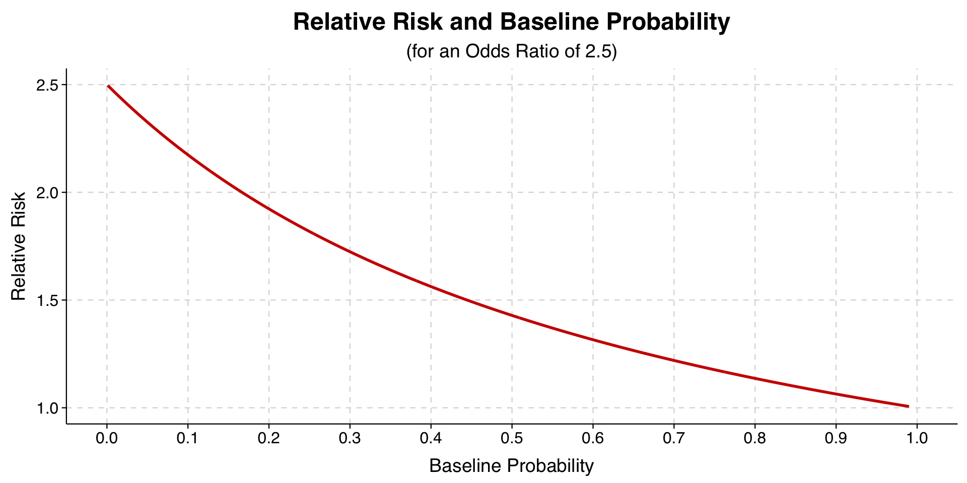
If we look at the formula of the relative risk, we can consider what happens as the baseline probability approaches 0 or 1:
\[\text{Relative Risk} = \frac{\text{Odds Ratio}}{(1-p_0) + (p_0 \times \text{Odds Ratio})}\]
As the baseline probability approaches 0, the \((1-p_0)\) term in the denominator approaches 1, while the \((p_0 \times \text{Odds Ratio})\) term approaches 0. The denominator thus approaches 1, meaning the relative risk approaches the odds ratio.
As the baseline probability approaches 1, the \((1-p_0)\) approaches 0, and the \((p_0 \times \text{Odds Ratio})\) term approaches the odds ratio. As a result, we end up dividing the odds ratio by the odds ratio, yielding 1.
As the baseline probability goes from 0 to 1, then, the relative risk goes from being equal to the odds ratio to being equal to 1.
Here is a plot that uses our example where the odds ratio was 2.5. The plot shows how the relative risk changes as the baseline probability changes.
# Create data frame with p0 values from 0.01 to 0.99
plotdf <- data.frame(p0 = seq(0.001, 0.990, by = 0.001))

# Calculate relative risk for each p0 value using the formula
# RR = OR / ((1-p0) + p0*OR)
plotdf <- plotdf %>%
  mutate(relative_risk = 2.5 / ((1-p0) + p0*2.5))

# Create the plot
ggplot(plotdf, aes(x = p0, y = relative_risk)) +
  geom_line(color = "red3", linewidth = 1) +
  labs(
    title = "Relative Risk and Baseline Probability",
    subtitle = "(for an Odds Ratio of 2.5)",
    x = "Baseline Probability",
    y = "Relative Risk"
  ) +
  scale_x_continuous(limits = c(0, 1), breaks = seq(0, 1, 0.1)) +
  scale_y_continuous(limits = c(1, 2.5)) +
  theme_tula() +
  theme(
    plot.title = element_text(hjust = 0.5),
    plot.subtitle = element_text(hjust = 0.5),
    panel.grid.minor = element_blank()
  )
For most methods of interpreting binary outcomes, switching which outcome category is coded as 0 or 1 reverses the value in some way, but the substantive gist of the interpretation would be the same.
Relative risk is different. After all, if we look at the probabilities of being a Democratic donor by a professor’s gender:
Mean of (rep_donor == "no")
────────┼─────────────────
    man │    Mean        N
────────┼─────────────────
  no    │    .968   28,342
  yes   │    .922   28,569
────────┼─────────────────
  Total │    .945   56,911
Then if we consider men vs. women, the relative risk is .922 / .968 = .95.
In other words, even though men were 2.4 times as likely to be Republican donors, they are only 5% less likely to be Democratic donors.
In practice, one typically sees relative risk used in contexts where the less frequent category is coded as 1 and the more frequent category is coded as 0.
In a model with covariates, one can be interested in the average relative risk, which computes the relative risk for each observation based on its baseline probability (i.e., based on its values of the explanatory variables).
We can do this in R using the avg_comparisons() function from the marginaleffects package.
model2 <- glm((rep_donor == "yes") ~ man + ivyplus + cpvi25_red,
             data = data, family = "binomial")

avg_comparisons(
  model2,
  variables = "man",
  comparison = "ratio"
)
 Estimate Std. Error    z Pr(>|z|)     S 2.5 % 97.5 %
     2.41     0.0954 25.2   <0.001 464.3  2.22   2.59

Term: man
Type: response
Comparison: mean(yes) / mean(no)
We can see that our estimated relative risk is 2.41. Very close to what we had before. A shorthand interpretation:
By “on average,” we mean we are averaging over everyone in our data based on their values of \(\texttt{ivyplus}\) and \(\texttt{cpvi25\_red}\).