# simulate values
count <- rpois(n = 1000000, lambda = 2.3)

# compute mean
mean(count)
[1] 2.300076The Poisson distribution relates the probability of a particular count of the number of times an event occurs to an underlying rate. For example, the state of California has a “Daily 3” lottery that involves picking a three digit sequence in order, so the rate of winning is 1 in 1000. However, if you play “Daily 3” a 1000 times, this doesn’t mean that you will win once: you might never win, or you might win twice. The Poisson distribution allows us to calculate the probability of winning the “Daily 3” a given times given the underlying rate.
The Prussian military became concerned about the number of cavalry soldiers killed (in peacetime) by getting kicked by a horse. The Prussians, who were pioneers in military organization, gathered data, and a statistician, Ladislaus Bortkiewicz, analyzed it.
Over a extended period of observation, some cavalry units had multiple deaths by horsekick, while many units had none. For 280 unit-years (14 units for each of 20 years), the data were like this:
| Deaths | # Unit-Years | Proportion |
|---|---|---|
| 0 | 144 | .514 |
| 1 | 91 | .325 |
| 2 | 32 | .114 |
| 3 | 11 | .039 |
| 4 | 2 | .007 |
There were two broad possibilities:
Bortkiewicz showed that if the units were simply unlucky, the data would be expected to follow a Poisson distribution. With the Poisson distribution, there is a overall rate at which the event occurs, denoted by \(\lambda\) (lambda). If all units have been exposed for the same amount of time, then \(\lambda\) the expected average count.
Given \(\lambda\), the probability of a unit observing count \(k\) under the Poisson distribution is:
\[ \Pr(y=k|\lambda) = \frac{\lambda^k e^{-\lambda}}{k!} \]
In the Prussian data, the average number of deaths per unit-year was .7. So the probability of a unit having no deaths in a year was:
\[ \begin{align} \Pr(y=0) & = \frac{.7^0 e^{-.7}}{0!} \\ \\ & = \frac{(1)(.497)}{(1)} \\ \\ & = .497 \\ \end{align} \]
Given the overall death rate of .7 soldiers per year, we would expect 49.7% of the units to have no deaths in a given year, which is consistent with what was observed. We can go through and calculate the probabilities for each of the observed counts and compare the expected proportions to the actual observed proportion of corps with each fatality count:
| Deaths | Observed | Expected |
|---|---|---|
| 0 | .514 | .497 |
| 1 | .325 | .348 |
| 2 | .114 | .121 |
| 3 | .039 | .028 |
| 4 | .007 | .004 |
| 5+ | 0 | .001 |
We can see that the observed and expected values here are close. From this, we would conclude we do not have reason to think that the units and years with higher counts was anything more than bad luck.
Now let’s imagine the case where there really was something going on with some Prussian cavalry units that made them have a higher risk of death. I created 4 new units (80 observations total) whose death total is actually just the death total for three of the real units combined. Including them in our dataset gives us the new values in the “Observed” column below:
| Deaths | Observed | Expected |
|---|---|---|
| 0 | .441 | .368 |
| 1 | .308 | .368 |
| 2 | .139 | .184 |
| 3 | .064 | .061 |
| 4 | .028 | .015 |
| 5 | .008 | .003 |
| 6 | .008 | .001 |
| 7+ | .003 | <.001 |
By happy coincidence, the new rate \(\lambda\) for the new dataset happens to be exactly 1. We can compare observed to expected proportions from a Poisson distribution in which \(\lambda\) is 1.
The deviations from expected under the Poisson distribution are bigger than before. Not only that, but they are bigger in a predictable way: there are more low (=0) counts and more high (>3) counts than expected, and fewer cases in the middle. In other words, the variance in the observed counts is more than what we would expect under the Poisson distribution.
There is a bigger substantive point here. When the data generating process is the same for all observations – when they all faced the same rate \(\mu\) of the outcome and the differences in the observed count is simply due to chance – the expected distribution of the outcome is Poisson. When there is heterogeneity in the data generating process – like different observations having different underlying values of \(\lambda\) – the distribution will have greater variance than Poisson.
Aside: What would it mean to have a variance for a count variable that is less than the mean? It can happen, and does. What it implies is a data generating process that creates more homogeneity in counts than what would be expected if the event simply occurred by random chance. Number of children is an example. Because of the (admittedly, waning) common preference for exactly two children, there are a larger number of counts of two children than one would expect given the Poisson distribution, and the variance is regularly less than the mean.
The normal distribution, for example, is defined by two parameters: one for its mean and one for its variance. Those two parameters are all you need to draw the normal distribution on a number line and calculate any associated probabilities.
For the Poisson: \(\lambda\) is the only parameter. \(\lambda\) is both the mean of the Poisson distribution and its variance. With the normal distribution, data can follow a normal distribution and be relatively squished together or relatively spread out. Not so with Poisson!
One can randomly simulate data that follows a poisson distribution with the rpoisson() function. I will arbitrarily use \(\mu = 2.3\) here.
I simulate values from the Poisson distribution using the rpois() function, and then I compute the mean:
# simulate values
count <- rpois(n = 1000000, lambda = 2.3)
# compute mean
mean(count)[1] 2.300076The mean is 2.3. Now, I will compute the variance:
# compute variance
var(count)
[1] 2.305179The variance is also 2.3. The mean and variable are both equal to the \(\lambda\) parameter.
I simulate data and generate summary statistics:
. clear all

. set obs 1000000
Number of observations (_N) was 0, now 1,000,000.

. gen count = rpoisson(2.3)

. sum, detail

                            count
-------------------------------------------------------------
      Percentiles      Smallest
 1%            0              0
 5%            0              0
10%            0              0       Obs           1,000,000
25%            1              0       Sum of wgt.   1,000,000

50%            2                      Mean           2.295481
                        Largest       Std. dev.       1.51462
75%            3             12
90%            4             12       Variance       2.294072
95%            5             12       Skewness       .6600804
99%            6             13       Kurtosis       3.438853
If you look at the above statistics from our simulated data, you will see that the mean and variance are both approximately 2.3. (Neither will be exactly 2.3 as a matter of random chance, but the larger our sample, the closer both will be.)
Below are some examples of the Poisson distribution for different values of \(\lambda\). In each case, the probabilities for each count are computed using the formula:
\[ \Pr(y=k|\lambda) = \frac{\lambda^k e^{-\lambda}}{k!} \]
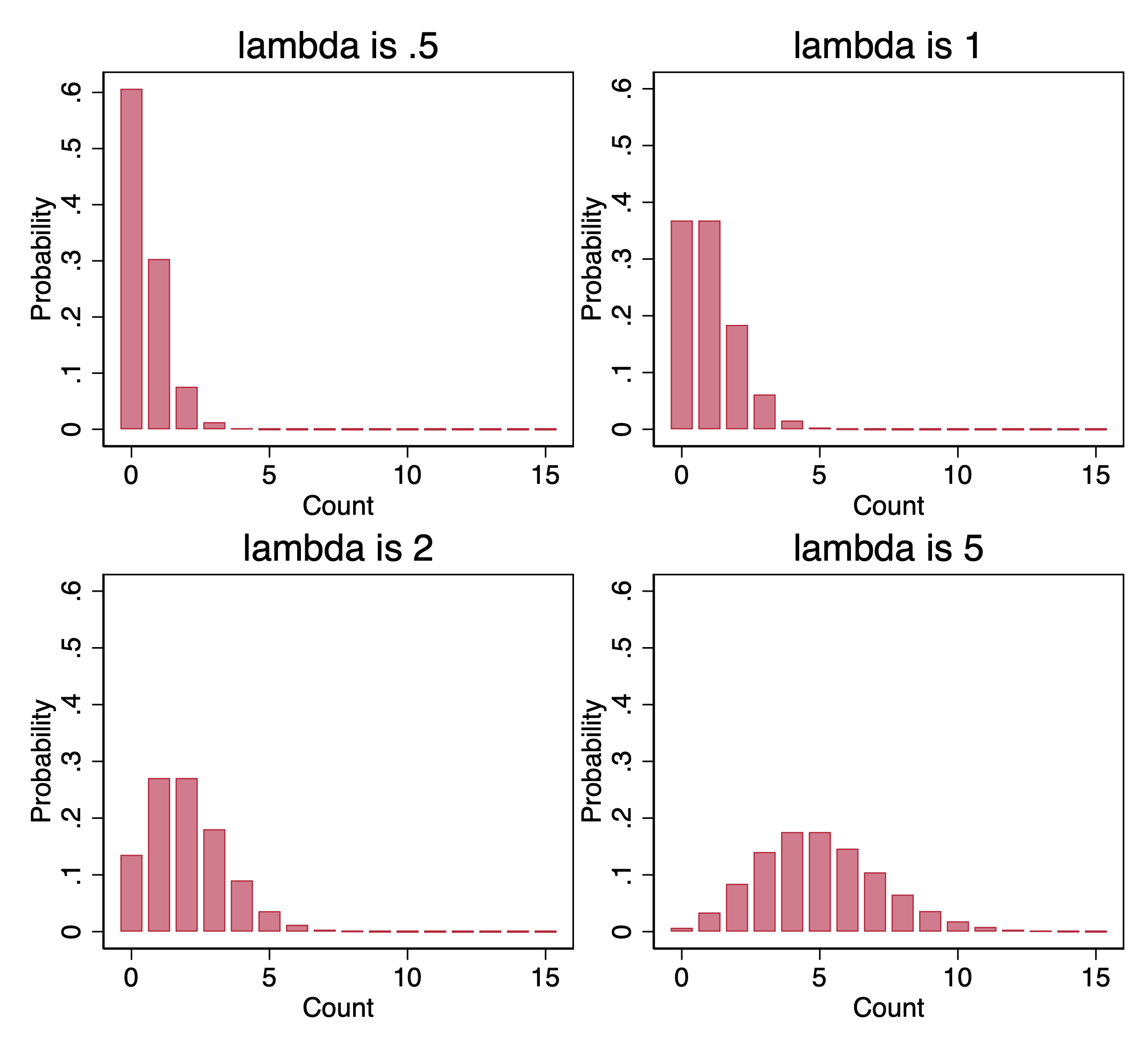
Notice that, for the examples where \(\lambda\) is an integer, the probabilities that \(y = \lambda\) and that \(y = \lambda - 1\) are the same. This might seem counterintuitive, as it might seem like \(y = \lambda\) should be more likely than \(y = \lambda - 1\) given that \(\lambda\) the mean.
But, consider, while counts can never be below zero, counts do not have any upper bound. So the Poisson distribution is asymmetric; more precisely, it is skewed to the right. That is, under the Poisson distribution, there will be some observations with more extreme values to the right of the mean than the most extreme values to the left of the mean, because to the left extreme values are constrained by zero.
A right-ward skew pulls the mean of a unimodal distribution up relative to its mode. In the case of Poisson, the rightward skew works out so that \(\Pr(y = \lambda) = \Pr(y = \lambda - 1)\) if \(\lambda\) is an integer. For example, if \(\lambda\) is 3 for an outcome that follows a Poisson distribution, the probability of observing a count of 2 will be exactly the same as the probability of observing a count of 3, and these will be the most likely counts observed in the data.
Skippable: Proof that \(\Pr(y=\lambda) = \Pr(y=\lambda-1)\) when \(\lambda\) is an integer. As indicated above, the probability that \(y = k\) in a Poisson distribution for any integer \(k\) is:
\[ \Pr(y=k) = \frac{\lambda^k e^{-\lambda}}{k!} \]
If \(\lambda\) is an integer, then the probability that \(y = \lambda\) is.
\[ \Pr(y=\lambda) = \frac{\lambda^\lambda e^{-\lambda}}{\lambda!} \]
So what we will prove is that the right hand side above is equal not just to \(\Pr(y=\lambda)\) but also \(\Pr(y=(\lambda-1))\).
Going back to the formula for the Poisson distribution and instead considering \(\Pr(y=(\lambda-1))\), we get:
\[ \Pr(y=(\lambda-1)) = \frac{\lambda^\left(\lambda-1\right) e^{-\lambda}}{(\lambda-1)!} \]
This probability is unchanged if we multiply it by 1, which here we express as \(\frac{\lambda}{\lambda}\) \[ \begin{align} \Pr(y=(\lambda-1)) & = \frac{\lambda}{\lambda} \frac{\lambda^\left(\lambda-1\right) e^{-\lambda}}{(\lambda-1)!} \\ \\ & = \frac{\left(\lambda \times \lambda^\left(\lambda-1\right)\right) e^{-\lambda}}{\lambda \times (\lambda-1!)} \end{align} \]
As part of the numerator, we have \(\lambda \times \lambda^\left(\lambda-1\right)\). If you have \(a^b\) and multiply it by \(a\), you get \(a^\left(b+1\right)\). So \(\lambda \times \lambda^\left(\lambda-1\right) = \lambda^\lambda\).
Meanwhile, in the denominator, we have \(\lambda \times (\lambda-1!)\). If we have \(a!\) and multiply it by \(a+1\), we have \(a+1\) factorial. So, \(\lambda \times (\lambda-1!) = \lambda!\)
Putting this together, then: \[ \begin{align} \Pr(y=(\lambda-1)) & = \frac{\lambda^\lambda e^{-\lambda}}{\lambda!} \\ \\ & = \Pr(y=\lambda) \end{align} \]