One will sometimes hear people talk about parametric, non-parametric, and semi-parametric statistical models. Definitions vary and would take us afield anyway. In general, parametric models make assumptions about the form of the relationship between the explanatory variables and the outcome. For example, in linear regression, we make an assumption of a linear relationship between the explanatory variable and outcome. Even though we can transform things and add parameters in order to model non-linear relationships via linear regression, there are still limits to the non-linearities we can model in a linear regression framework.
In a parametric survival analysis model, we need to specify the basic shape of the hazard function we will use. Later, when we discuss the Cox proportional hazards model, which is semi-parametric and does not requires us to specify any shape for the hazard function.
Here we will introduce the simplest parametric survival analysis model, which is the exponential regression model.
The model
In the exponential regression model, we assume the hazard function is constant. That is, the hazard can differ for different values of the explanatory variables, but it does not vary over time. When the hazard is constant over time, the distribution of the survival function is exponential.
The hazard function for exponential regression is:
That the above implies a constant hazard can be seen in how the right hand side does not include \(t\). Note also that this is similar to a regression model with a logged outcome, only here our outcome is the hazard.
The cumulative hazard in this case is just the hazard times \(t\):
Aside: Baseline hazard. In this and other parametric models we will consider, \(\mathbf{x}\mathbf{\beta}\) includes an intercept term \(\beta_0\). \(\beta_0\) is sometimes called the baseline hazard. This is the estimated hazard when all the explanatory variables are 0.
Example
Using the animal shelter data, we will fit a model of time to adoption for cats using two explanatory variables: color and age at intake.
── Attaching core tidyverse packages ──────────────────────── tidyverse 2.0.0 ──
✔ dplyr     1.2.0     ✔ readr     2.2.0
✔ forcats   1.0.1     ✔ stringr   1.6.0
✔ ggplot2   4.0.2     ✔ tibble    3.3.1
✔ lubridate 1.9.5     ✔ tidyr     1.3.2
✔ purrr     1.2.1
── Conflicts ────────────────────────────────────────── tidyverse_conflicts() ──
✖ dplyr::filter() masks stats::filter()
✖ dplyr::lag()    masks stats::lag()
ℹ Use the conflicted package (<http://conflicted.r-lib.org/>) to force all conflicts to become errors
library(haven)library(survival)library(modelsummary)# Load data# Note: austin_animals_stset.dta was stset in Stata, so time = _t and event = _ddat <-read_dta("../dta/austin_animals_stset.dta") %>%filter(cat ==1) %>%mutate(agecat =as_factor(agecat))# Create color categoriesdat <- dat %>%mutate(black = color1 =="Black"& (color2 ==""| color2 =="Black"),white = color1 =="White"& (color2 ==""| color2 =="White") ) %>%mutate(color4cat =case_when( black ~"black", white ~"white",!black &!white & color2 ==""~"other one-color",!black &!white & color2 !=""~"multicolor" ) ) %>%mutate(color4cat =factor(color4cat,levels =c("black", "white", "other one-color", "multicolor")) )# Fit exponential regression model (AFT parameterization)# _t = analysis time, _d = failure indicator (from Stata stset)mod_exp <-survreg(Surv(`_t`, `_d`) ~ color4cat + agecat,data = dat, dist ="exponential")# Display model summarysummary(mod_exp)
Call:
survreg(formula = Surv(`_t`, `_d`) ~ color4cat + agecat, data = dat,
    dist = "exponential")
                           Value Std. Error      z       p
(Intercept)               3.8778     0.0342 113.26 < 2e-16
color4catwhite           -0.4316     0.1226  -3.52 0.00043
color4catother one-color -0.1447     0.0372  -3.89 9.9e-05
color4catmulticolor      -0.1213     0.0385  -3.15 0.00162
agecat5-11 months        -0.2007     0.0369  -5.43 5.5e-08
agecat1-3 years           0.2521     0.0371   6.79 1.1e-11
agecat> 3 years           0.5572     0.0325  17.16 < 2e-16

Scale fixed at 1

Exponential distribution
Loglik(model)= -36627.7   Loglik(intercept only)= -36847.5
    Chisq= 439.65 on 6 degrees of freedom, p= 8.3e-92
Number of Newton-Raphson Iterations: 6
n=17932 (7708 observations deleted due to missingness)
To convert from the AFT parameterization (which survreg uses) to the proportional hazards parameterization (as shown in the Stata output above), we exponentiate the coefficients and take their reciprocal: exp(-coef). The AFT coefficients represent acceleration factors for survival time.
From the signs of the coefficients, we can see that black and older cats have the lowest rate of adoption. Beyond this, to interpret the coefficients, we would want to exponentiate the coefficients.
Stata: hazard ratios. In exponential regression, hazard ratios are provided by default. (I used the \(\texttt{nohr}\) option in the example above to obtain the untranformed coefficients.) Whether streg provides transformed coefficients or not varies depends on the specified distribution. If a distribution supports hazard ratios, they can be obtained with the \(\texttt{hr}\) option.
. streg, hr allbaselevels

Exponential PH regression

No. of subjects =     17,932                            Number of obs = 17,932
No. of failures =      7,552
Time at risk    = 365,396.49
                                                        LR chi2(6)    = 439.65
Log likelihood = -14731.19                              Prob > chi2   = 0.0000

----------------------------------------------------------------------------------
              _t | Haz. ratio   Std. err.      z    P>|z|     [95% conf. interval]
-----------------+----------------------------------------------------------------
       color4cat |
          black  |          1  (base)
          white  |   1.539647   .1887035     3.52   0.000     1.210865    1.957704
other one-color  |   1.155708   .0429568     3.89   0.000     1.074508    1.243045
     multicolor  |   1.129012   .0434688     3.15   0.002      1.04695    1.217506
                 |
          agecat |
     0-4 months  |          1  (base)
    5-11 months  |   1.222312   .0451548     5.43   0.000     1.136939    1.314097
      1-3 years  |   .7771754   .0288501    -6.79   0.000     .7226382    .8358284
      > 3 years  |   .5728351   .0185994   -17.16   0.000     .5375167    .6104742
                 |
           _cons |   .0206961   .0007086  -113.26   0.000     .0193529    .0221326
----------------------------------------------------------------------------------
Note: _cons estimates baseline hazard.
# Extract coefficients and convert to hazard ratios# In the AFT parameterization, hazard ratios are exp(-coef)coefs <-coef(mod_exp)hr <-exp(-coefs)# Display hazard ratiosprint(hr)
             (Intercept)           color4catwhite color4catother one-color
              0.02069613               1.53964750               1.15570838
     color4catmulticolor        agecat5-11 months          agecat1-3 years
              1.12901187               1.22231230               0.77717536
         agecat> 3 years
              0.57283514
In the AFT parameterization used by survreg, hazard ratios are obtained by exponentiating and inverting the coefficients: exp(-coef). This gives us the proportional hazards parameterization that matches the Stata output above. For instance, white cats have a hazard ratio of approximately 1.54 compared to black cats, indicating a 54% higher adoption rate.
Examples of how these hazard ratios can be interpreted are:
White cats have a 54% higher rate of adoption than white cats.
Cats that are 5-11 months when they enter the animal shelter are adopted at a 22% higher rate than younger cats.
Cats that are more than 3 years old when they enter the animal shelter are adopted at a 43% lower rate than cats that were 0-4 months old when entering the shelter.
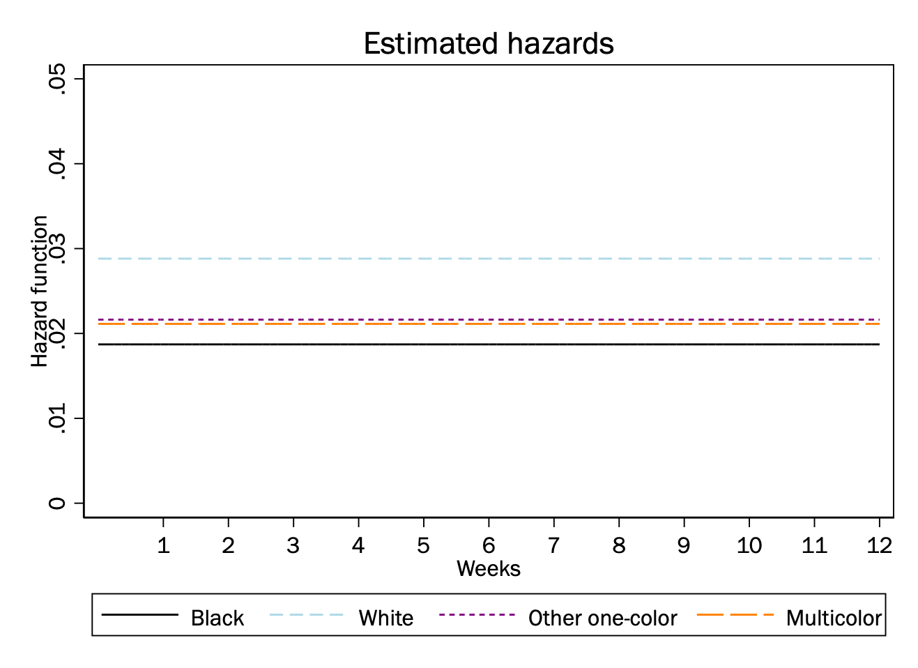
If we graph the implied hazard functions, we can see clearly the constant hazard assumption and what it means for a categorical variable to have a proportional relationship to the hazard.
For example, above we showed that the results indicate that the hazard rate is 54% higher for white cats than black cats. In the above graph, we can see that the estimated hazard for black cats is constant at around .19 and for white cats it is around .29, for the reported difference of 54%.
Interpreting results in terms of estimated median survival time
For parametric survival time models, we can also estimate quantities like the predicted median survival time: that is, the time at which an observation with a given covariate profile is expected to have a 50% chance of survival.
. margins i.color4cat, predict(median time)

Predictive margins                                      Number of obs = 17,932
Model VCE: OIM

Expression: Predicted median _t, predict(median time)

----------------------------------------------------------------------------------
                 |            Delta-method
                 |     Margin   std. err.      z    P>|z|     [95% conf. interval]
-----------------+----------------------------------------------------------------
       color4cat |
          black  |   38.05835   1.286191    29.59   0.000     35.53746    40.57924
          white  |   24.71887   2.913793     8.48   0.000     19.00794     30.4298
other one-color  |   32.93076   .5451005    60.41   0.000     31.86238    33.99913
     multicolor  |   33.70943   .6520134    51.70   0.000     32.43151    34.98736
----------------------------------------------------------------------------------
# Predict median survival time for each color category# Create prediction gridpred_grid <-expand.grid(color4cat =levels(dat$color4cat),agecat =levels(dat$agecat)[1] # hold at base category (0-4 months))# Predict median survival timesmedian_times <-predict(mod_exp, newdata = pred_grid, type ="quantile", p =0.5)results <- pred_grid %>%mutate(median_time = median_times) %>%select(color4cat, median_time)print(results)
        color4cat median_time
1           black    33.49164
2           white    21.75280
3 other one-color    28.97932
4      multicolor    29.66456
The predicted median time to adoption varies by color: black cats have the longest expected time to adoption (approximately 38 days), while white cats have the shortest (approximately 25 days).
We could intepret the above results as indicating that: - After adjusting for age at intake, the median expected time to adoption for a black cat is 38 days, while for white cats it is 25 days.
To give a different example, we can look at whether the tendency for black cats to be adopted later also extends to black dogs. If we look at the model coefficients, we would see that there is a statistical interaction, meaning that the association between color and adoption is not the same for cats and dogs. We will here use margins to show us the difference in terms of median time to adoption:
# Load full dataset (both cats and dogs)dat_full <-read_dta("../dta/austin_animals_stset.dta") %>%filter(cat ==1| dog ==1)# Create black color indicatordat_full <- dat_full %>%mutate(black = color1 =="Black"& (color2 ==""| color2 =="Black"),cat_ind =as.integer(cat ==1),dog_ind =as.integer(dog ==1) )# Fit model with interaction between black and cat# _t = analysis time, _d = failure indicator (from Stata stset)mod_interact <-survreg(Surv(`_t`, `_d`) ~ black * cat_ind,data = dat_full, dist ="exponential")# Create prediction grid for all combinationspred_grid2 <-expand.grid(black =c(FALSE, TRUE),cat_ind =c(FALSE, TRUE))# Predict median survival timesmedian_times2 <-predict(mod_interact, newdata = pred_grid2, type ="quantile", p =0.5)results2 <- pred_grid2 %>%mutate(animal =ifelse(cat_ind, "cat", "dog"),color =ifelse(black, "black", "not black"),median_time = median_times2 ) %>%select(animal, color, median_time)print(results2)
  animal     color median_time
1    dog not black    21.24641
2    dog     black    21.36846
3    cat not black    30.63328
4    cat     black    36.18289
For dogs, the median adoption time is approximately three weeks regardless of color. For cats, black cats have a longer median adoption time (about 36 days) compared to non-black cats (about 31 days).
Looking at these results, we can see that for dogs, the median time for adoption is about three weeks and whether the dog is black or not makes no difference. For cats, on the other hand, the median time to adoption for black cats is about six days longer than it is for cats that are not black.