Proportional hazards versus accelerated failure time

There are two primary strategies for how we might model how a duration outcome is associated with explanatory variables, known as the proportional hazards and the accelerated failure-time approaches.

When the hazard rate is constant within an individual, these two approaches are effectively the same. When the hazard varies, they are usually not. We will consider a toy example in which the hazard is constant as a way of explaining the distinction.

Simple example

California has a twice-daily “Daily 3” lottery drawing in which a three digit sequence is selected. There are 1,000 possible combinations (ranging from 0-0-0 to 9-9-9). A person playing the lottery has a 1 in 1000 chance of winning each and every time they play, and the chance of winning has absolutely nothing to do with success or failure in the past.

We can consider three different groups of players:

Group A: Plays the Daily 3 drawing once per day.
Group B: Plays the Daily 3 drawing twice per day.
Group C: Plays the Daily 3 drawing every other day.

As long as a player persists in playing, they will eventually win. Nevertheless, we can expect that members of Group B, on average, will win sooner than members of Group A, and likewise members of Group A will win sooner on average than members of Group C.

The proportional hazards approach

In the proportional hazards approach, explanatory variables are understood as having some multiplicative relationship to the hazard rate. The hazard in our case may be seen as the risk of winning the lottery on a particular day.

Say we used \(h_{BASELINE}(t)\) to equal a baseline hazard; in our case, we will say the baseline hazard is the hazard for Group A:

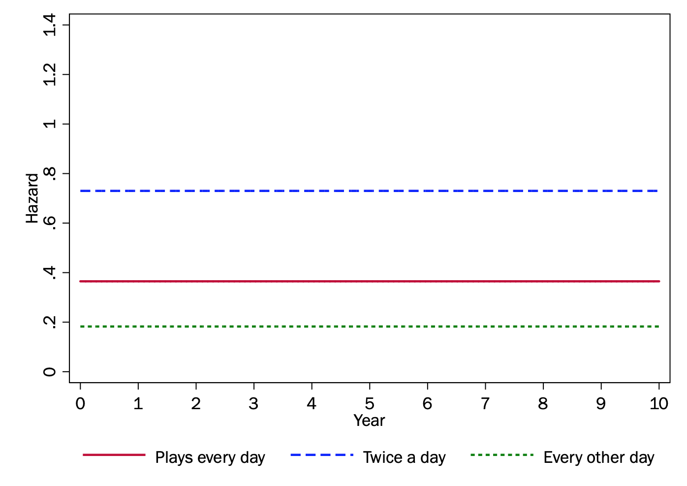
\[ h_A(t) = h_{0}(t) = 1/1000 = .001 \textrm{per day } \textrm{(cumulating to }.365\textrm{ in a year)} \]

For Group B, the hazard would be twice the baseline, and for Group C, the hazard would be half the baseline.

\[ \begin{align} h_B(t) & = 2 \times h_{0}(t) = 2/1000 = .002 \\ \\ h_C(t) & = .5 \times h_{0}(t) = .5/1000 = .0005 \\ \end{align} \]

In our toy example, things are simple because the hazard is otherwise constant: the baseline hazard is always .001 per day, or each day 1 in 1000 members of Group A will win.

However, the hazard could vary. Say that every December the State of California runs a special Christmas version of the game where two winning combinations are drawn each drawing instead of one. Everybody’s chance of winning effectively doubles. But, the hazard for Group B remains twice as big as the hazard for Group A, and the hazard for Group C remains half the size. In a proportional hazards model, the baseline hazard may vary over time, but the proportional difference of a group (or combination of explanatory variables) remains the same.

In a proportional hazard model, exponentiating coefficients yields a hazard ratio. The hazard ratio \(exp(\beta)\) indicates the multiplicative change from the baseline change for a one-unit increase in the variable (or, for a categorical explanatory variable, the multiplicative change associated with being a member of a given category vs. the base category).

The accelerated failure-time approach

In the proportional hazards approach, explanatory variables are modeled in terms of their effect on the hazard, and their consequences for the survival curve is a byproduct of this effect on the hazard. Increasing the hazard will make the survival curve steeper, which makes the expected time to the occurrence of the event sooner. In the accelerated failure time approach, on the other hand, we model the relationship between explanatory variables and the expected time of the event happening directly.

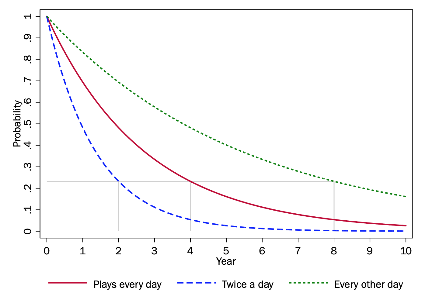
In the accelerated failure-time approach, explanatory variables accelerate or decelerate the failure process. The survival curve has the same basic shape across groups, but explanatory variables speed up or slow down how quickly groups traverse that survival curve. In effect, the curve is either scrunched to the left (speeding up time) or stretched out to the right (slowing time down) by some proportional amount.

Compared to the baseline of Group A, the failure process happens twice as quickly for Group B and only half as fast for Group C. Putting it another way, we would expect Group B to reach the same points in the survival curve (like, say, the time at which one has a 50% chance of having won) in half the time as Group A, whereas Group C would take twice as long reach the same points as Group A.

Which should you use?

Ultimately this is a substantive question, although I would note that proportional hazard models are more popular, probably easier to intepret, and at least to me are more easily to substantially conceptualize, as I tend to think of the hazard as fundamental for duration outcomes and survival as a byproduct of probabilistic success given the hazard.

In that light, it is worth mentioning that the clearest analogue of using (logged) linear regression for a survival outcome is the parametric lognormal regression model, and this is an accelerated failure-time model.