Survival analysis: key principles
This page describes several basic concepts at the heart of survival analysis.
Survival
- When we model outcome events, we are usually interested in the “age” of the observation rather than calendar time. That is, we can think of each individual as having a clock whose time \(t\) starts at 0 at the time of their “birth” (this is sometimes called the origin).
- Of course, the origin might not be literal birth. For example, if we are studying divorce as our failure event, “birth” would be marriage and “age” would be the duration of marriage. That is, the origin corresponds to when the possibility of the outcome event happening begins–the time at which an observation first becomes at risk.
- When we say that \(t\) is the same for two observations, we mean they are the same “age”, not the same calendar date.
- At every point during their “lives”, individuals are at some risk of the outcome event occurring.
- Survival to a particular point in time \(t\) means having faced whatever level(s) of risk up to \(t\) without the event happening.
Survival curve
The survival curve, also called the survivor function, shows the proportion of the population surviving to a given point \(t\). A survival curve never increases over time.
Wikipedia’s example with survival curves provides a biological example of survival curves for different types of species:
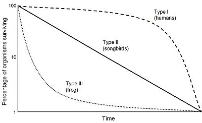
The \(x\)-axis here is the age of an individual member of the species. In all three species – like everything else – the probability of survival declines with age. The graph is meant to illustrate how, for example, for frogs most offspring die young and only a few survive into adulthood. In contrast, (esp. contemporary) humans more often survive to a reasonably old age and the survivor rates decline sharply over a fairly compressed period relative to overall lifespan.
Here are some examples of survivor curves for human mortality in Switzerland:
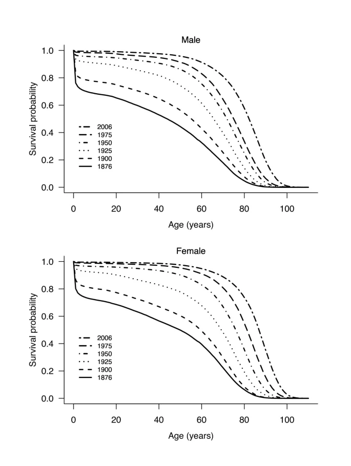
Here the \(x\)-axis values are specific ages, and the different lines are different birth cohorts. This graph involves making demographic projections, which is outside our scope. But these graphs show how, for example, for people born in 1876, survival to age 80 was relatively rare, but for cohorts born in 2006, most people are expected to survive into their 80s.
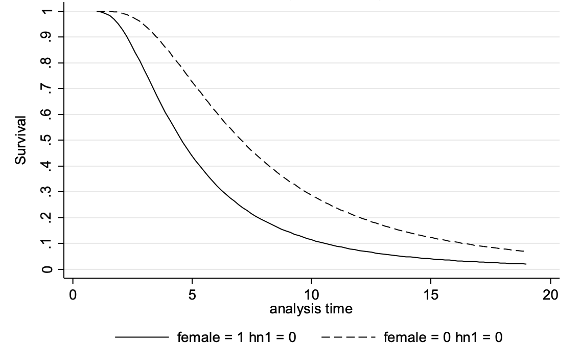
Here is the example of marriage in the Wisconsin Longitudinal Study data (respondents born ~1939), in which analysis time starts at age 16 (but the sample includes only those who were unmarried as high school seniors):
Hazard
- The risk of the failure event occurring at some interval \(t-1\) to \(t\), conditional on the observation surviving to \(t-1\), is called the hazard. The hazard of death at age 70 is not simply the probability of dying at age 70; it is the probability of somebody, having reached their 70th birthday, dying before their 71st birthday.
- The hazard may differ systematically for different individuals. If it does, then on average we would expect the event to happen sooner to individuals with higher hazards.
- The hazard may also change for an individual because their characteristics change. This is like the example above where we thought that the hazard of mortality might increase when someone is widowed.
Hazard function
The hazard may also vary with the passage of time. The hazard function characterizes how the hazard changes over time.
- A constant hazard means that the risk of the event does not change over time. For example, consider a person who always buys a daily game lottery ticket. Their chance of winning is the same each day.
- An increasing hazard means the event is increasingly likely to happen as time passes (conditional on it not having happened yet). Throughout adulthood, the hazard of dying increases. The risk of somebody who turns 100 dying before their 101st birthday is higher than the risk of somebody who turns 90 dying before their 91st birthday, which in turn is higher than the risk for somebody who turns 80 dying before their 81st birthday, and so on.
- A decreasing hazard means the event is decreasingly likely to happen as time passes (conditional on it not having happened yet). In infancy, the hazard of dying decreases. The greatest risk for postnatal infant mortality is on the first day of life. For a baby who makes it through Day 1, the risk of dying on Day 2 is less, and, for those who make it through that, the risk of dying on Day 3 is still less.
- A non-monotonic hazard is a hazard that is increasing at some points in time and decreasing at other points. Mortality is like this, since the hazard decreases in infancy and increases through adulthood. Something like marriage is a different example, where the hazard of marrying in the following year increases through one’s teens and early twenties, and, for those who haven’t married, decreases through one’s thirties and beyond. (Exactly where the hazard switches from increasing to decreasing is itself something that varies across sex, subgroup, and society.)
The WLS marriage hazard plot provides an example of a non-monotonic hazard, namely:
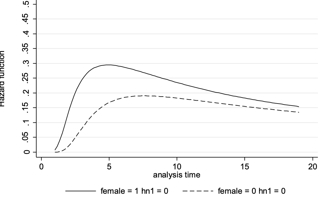
In the WLS data, the hazard of marrying first increases, and then, after peaking at age 21 for women and 23 for men, decreases.
Spell arrangement of survival data
Each individual in survival data is usually represented by multiple rows. Each row is a spell. A spell is a period of stability for the individual in terms of the variables germane to our analyses.
A spell ends for one of the following reasons: 1. The outcome event happens. 2. One of our explanatory variables changes. 3. The observation stops being observed (or otherwise leaves the pool of observations at risk, either temporarily or permanently).
Let’s go through some examples of spell data from data on duration of marriage. The failure event is divorce (\(\texttt{divorce}\)). We are interested in the effect of children on the risk of divorce, so that is a time-varying explanatory variable (\(\texttt{kids}\)). The variable \(\texttt{agemarried}\) is the age at which the respondent married, and \(\texttt{ageendspell}\) is the age at which the spell ends.
  |    id   spell  agemarried  ageendspell   kids   divorce |
  | 16347       1      27.296        33.79      0         1 |
This respondent was married at age 27.296 and divorced (with no kids) at age 33.79.
  |    id   spell  agemarried  ageendspell   kids   divorce |
  | 16349       1      21.498         26.5      0         0 |
This respondent was married at age 21.498. They were still married at age 26.5, when they stopped being observed for whatever reason. (This is an example of a censored observation.)
  |    id   spell  agemarried  ageendspell   kids   divorce |
  | 16358       1      17.667       18.915      0         0 |
  | 16358       2      17.667       26.001      1         0 |
  | 16358       3      17.667       31.666      2         0 |
  | 16358       4      17.667       37.872      3         1 |
This respondent was married at age 17.667. They had their first child at age 18.915, their second child at age 26.001, and their third child at age 31.666. They were divorced at age 37.872.
  |    id   spell  agemarried  ageendspell   kids   divorce |
  | 16364       1      30.582       31.329      0         0 |
  | 16364       2      30.582       53.689      1         0 |
  | 16364       3      30.582       56.334      2         0 |
This respondent married at age 30.582. They had their first child at age 31.329 and their second child at age 53.689. They were still married when they stopped being observed (for whatever reason) at age 56.334.
Arranging data into spells
R’s survival package has functions to help arrange data into spells. The Surv() function creates a survival-data object for analysis. The most important functions for splitting rows into spells are tmerge() and survSplit().
Stata has commands to help arrange data into spells. Typing \(\texttt{help st}\) will provide an introduction to these, and there is also much useful guidance online.