Uncertainty and maximum likelihood estimation

All else being equal, when you increase the sample size of a study, the uncertainty in your estimates decreases.

We can illustrate this using the Titanic data by making versions of the data with multiple copies of each observation. For example, our 1309-passenger dataset becomes 5236 “passengers” when we include 4 copies of each. I also made versions with 16 and 64 copies.

Below are the logit results. Each cell includes the logit coefficient with the standard error in parentheses. At the bottom is the log-likelihood of the model estimates.

Expand for code that loads packages and data

library(tidyverse)
library(haven)
library(tulaverse)
library(modelsummary)

titanic <- read_dta("../dta/titanic_passengers.dta") %>%
  mutate(pclass = relevel(as_factor(pclass), ref = "3rd"))

Expand to show code to create datasets, fit models, and show results

# create copies of data
titanic_4x <- titanic %>% 
  slice(rep(1:n(), each = 4))
titanic_16x <- titanic_4x %>% 
  slice(rep(1:n(), each = 4))
titanic_64x <- titanic_16x %>% 
  slice(rep(1:n(), each = 4))

# fit models
model <- glm(survived ~ pclass + male + child, 
                  family = binomial(link = "logit"), 
                  data = titanic)
model_4x <- glm(survived ~ pclass + male + child, 
                  family = binomial(link = "logit"), 
                  data = titanic_4x)
model_16x <- glm(survived ~ pclass + male + child, 
                  family = binomial(link = "logit"), 
                  data = titanic_16x)
model_64x <- glm(survived ~ pclass + male + child, 
                  family = binomial(link = "logit"), 
                  data = titanic_64x)

modelsummary(
  list("Orig N" = model, "4x" = model_4x, "16x" = model_16x, "64x" = model_64x),
  gof_map = list(
    list("raw" = "nobs",   "clean" = "N",               "fmt" = 0),
    list("raw" = "logLik", "clean" = "Log-Likelihood",  "fmt" = 3)
  ),
  fmt = 3
)

	Orig N	4x	16x	64x
(Intercept)	0.205	0.205	0.205	0.205
	(0.129)	(0.064)	(0.032)	(0.016)
pclass1st	1.862	1.862	1.862	1.862
	(0.176)	(0.088)	(0.044)	(0.022)
pclass2nd	0.898	0.898	0.898	0.898
	(0.180)	(0.090)	(0.045)	(0.023)
male	-2.499	-2.499	-2.499	-2.499
	(0.148)	(0.074)	(0.037)	(0.019)
child	1.085	1.085	1.085	1.085
	(0.229)	(0.115)	(0.057)	(0.029)
N	1309	5236	20944	83776
Log-Likelihood	-617.293	-2469.174	-9876.695	-39506.780

----------------------------------------------------------------
                   Orig N           4x          16x          64x
                     b/se         b/se         b/se         b/se
----------------------------------------------------------------
survived                                                        
1.pclass            1.862        1.862        1.862        1.862
                  (0.176)      (0.088)      (0.044)      (0.022)
2.pclass            0.898        0.898        0.898        0.898
                  (0.180)      (0.090)      (0.045)      (0.023)
male               -2.499       -2.499       -2.499       -2.499
                  (0.148)      (0.074)      (0.037)      (0.019)
child               1.085        1.085        1.085        1.085
                  (0.229)      (0.115)      (0.057)      (0.029)
_cons               0.205        0.205        0.205        0.205
                  (0.129)      (0.064)      (0.032)      (0.016)
----------------------------------------------------------------
N                    1309         5236        20944        83776
ll               -617.293    -2469.174    -9876.695    -3.95e+04
----------------------------------------------------------------

Things to notice in this table:

The logit coefficients are exactly the same. This makes sense given that the larger datasets are just multiple copies of the original dataset.
The standard errors of the coefficients decrease as the sample size gets larger. More specifically, each time we quadruple the size of our sample, the standard error is reduced by half.

This is a basic rule of thumb about sample size and precision: in order to double your precision (i.e., cut your uncertainty in half), you need to quadruple your sample size. The reason why is that the standard error is inversely proportional to the square root of the sample size, and 2 is the square root of 4.

The log-likelihood for the 4x sample is exactly 4 times that of the original N, and so on. This makes sense because the model log-likelihood is the sum of the log-likelihoods for each individual observation, so when the sample size doubles, we are adding twice as many individual log-likelihoods together to get the log-likelihood for the sample.

Likelihood function and uncertainty

In the example above, the estimate for \(\beta_{\texttt{child}}\) is 1.085. Again, because 1.085 is the maximum likelihood estimate, constraining the coefficient for child to any other value would produce a worse log-likelihood.

We can do exactly that: try out different candidate values for the \(\beta_{\texttt{child}}\) and compute the implied log-likelihood of the model.

What we will plot here is the difference between the maximum log-likelihood (when \(\beta_{\texttt{child}}\) is 1.085) and the log-likelihoods we get for other candidate values for \(\beta_{\texttt{child}}\).

Expand for code that computes log-likelihoods and draws plot

calc_likelihood <- function(data, beta_range) {
  # First, check if child is a factor and convert to numeric if needed
  if(is.factor(data$child)) {
    # Convert factor to numeric (0/1)
    # Assuming child is coded as "Yes"/"No" or similar
    data$child_numeric <- as.numeric(data$child) - 1
  } else {
    # If already numeric, just use as is
    data$child_numeric <- data$child
  }
  
  # Initial model
  full_model <- glm(survived ~ factor(pclass) + male + child_numeric, 
                   family = binomial(link = "logit"), 
                   data = data)
  
  max_ll <- logLik(full_model)
  
  # Create results dataframe
  results <- data.frame()
  
  for (beta in beta_range) {
    # Create model with constraint
    constrained_model <- glm(survived ~ factor(pclass) + male + offset(beta * child_numeric), 
                            family = binomial(link = "logit"), 
                            data = data)
    
    # Calculate distance from max likelihood
    ll_diff <- as.numeric(max_ll - logLik(constrained_model))
    
    # Add results
    results <- rbind(results, data.frame(beta = beta, ll = ll_diff))
  }
  
  return(results)
}

beta_range <- seq(0, 2, by = 0.005)
results_1 <- calc_likelihood(titanic, beta_range)
results_1$model <- 1

ggplot(results_1, aes(x = beta, y = -ll)) +
   geom_line(data = subset(results_1, ll <= 10), color="red3") +
   geom_vline(xintercept = 1.085, linetype = "dashed", color = "grey") +
   labs(y = "Distance from Maximum Likelihood") +
   theme_tula()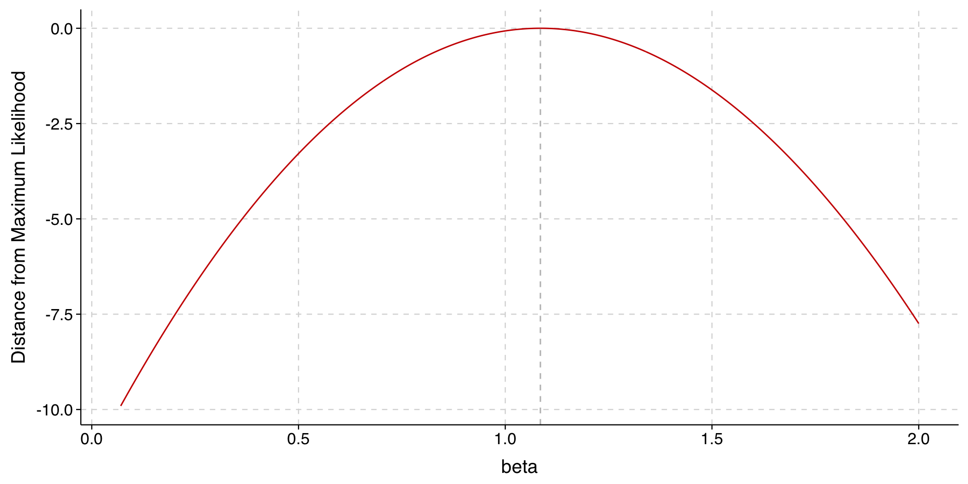

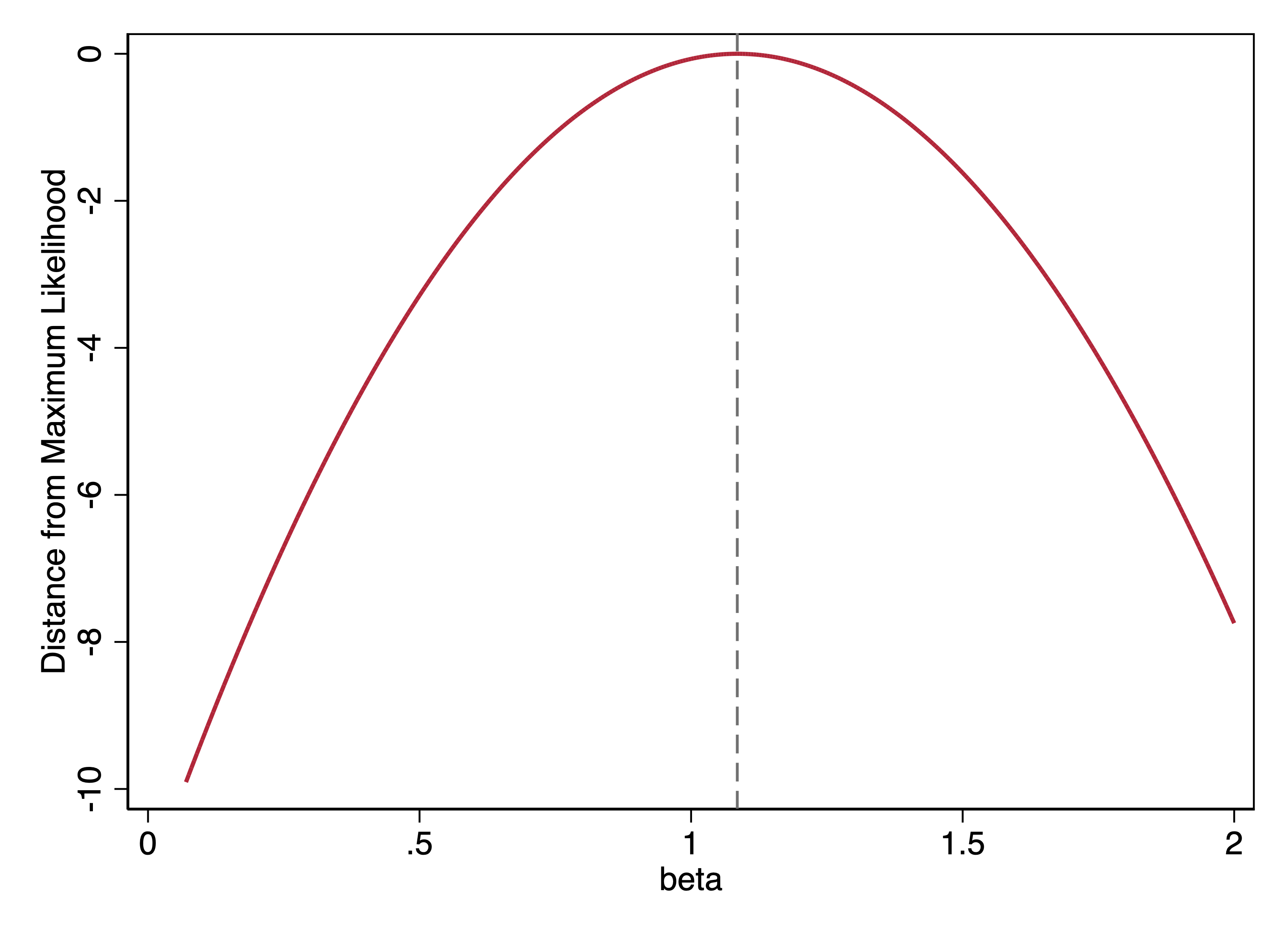
This is a graph of the likelihood function for our data and model with respect to \(\texttt{child}\).

On the \(y\)-axis, instead of the log-likelihood, I show the (negative) difference between the log-likelihood for the candidate beta and the maximum. At the maximum likelihood estimate of 1.085, \(y = 0\). At other values, \(y < 0\), where the farther one gets from 1.085, the larger the difference gets.

Here is the same graph, now adding the likelihood functions for our data with 4, 16, or 64 copies of each observation.

Expand for code that computes log-likelihoods and draws plot

results_2 <- calc_likelihood(titanic_4x, beta_range)
results_3 <- calc_likelihood(titanic_16x, beta_range)
results_4 <- calc_likelihood(titanic_64x, beta_range)

results_2$model <- 2
results_3$model <- 3
results_4$model <- 4

all_results <- rbind(results_1, results_2, results_3, results_4) %>%
  mutate(ll = -ll)

ggplot(all_results, aes(x = beta, y = ll, color = factor(model))) +
   geom_line(data = subset(all_results, ll >= -10)) +
   geom_vline(xintercept = 1.085, linetype = "dashed", color = "grey") +
   labs(y = "Distance from Maximum Likelihood") +
   scale_color_manual(values = c("red3", "blue", "darkgreen", "orange"),
                      labels = c("Original N", "4x", "16x", "64x")) +
   theme_tula() +
  theme(
    legend.position.inside = c(0.05, 0.95), # Positions legend inside upper left
    legend.justification = c(0, 1),   # Anchors the legend to its top-left corner
    legend.background = element_rect(fill = "white", color = NA),
    legend.title = element_blank()    # Removes the legend title
  )

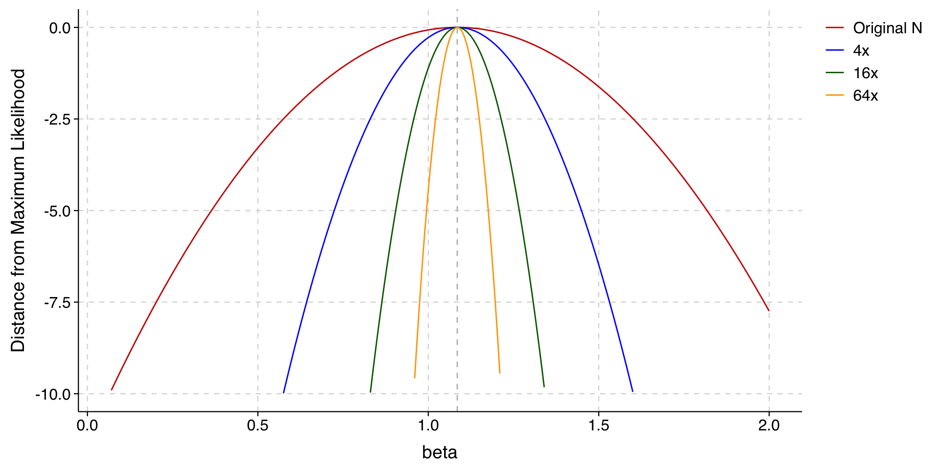
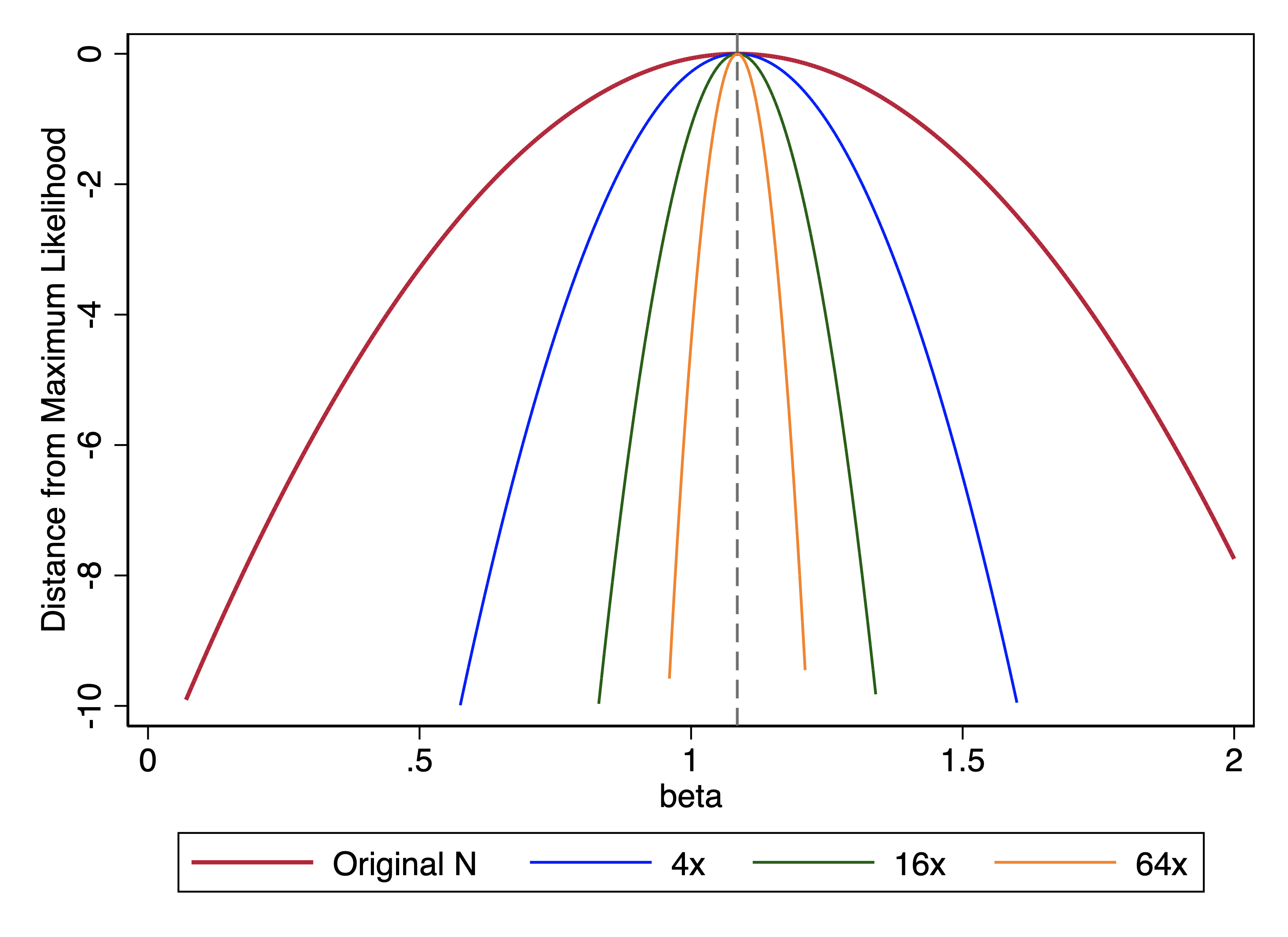
The maximum likelihood estimate is the same in all cases. But, as the sample gets larger, the function gets steeper (narrower around the point estimate).

At any given value on the \(y\)-axis, whenever we quadruple the sample, we make the likelihood function twice as narrow (i.e., we halve its width).

With maximum likelihood estimation, the maximum of the likelihood function provides our point estimate, and the steepness of the likelihood function is the basis for measuring uncertainty due to sampling variation. In a nutshell:

steeper likelihood function, which means
less uncertainty, which means
smaller standard errors, which means
larger z- or chi-squared statistics, which means
smaller p-values