Expand to show code to open data
library(tidyverse)
library(tulaverse)
library(modelsummary)
library(survival)

oscars_raw <- read_csv("../csv/oscars.csv")Multinomial logit models are often used to model choices that are an unordered outcome. Explanatory variables reflect characteristics of the chooser, and the model coefficients relate those explanatory variables to the chance that a particular outcome is chosen over its alternatives.
We can also have situations in which the characteristics of the available choices vary.
The example we will consider involves winners of the acting awards at the Oscars. We might be interested in predicting who wins out of a set of nominees. Predictors we might consider include:
Our outcome will be whether or not a given nominee wins the Oscar. This might seem like a problem to be addressed via a simple binary logit model, but it isn’t. Among a set of Oscar nominees, one of them must win. For a set of nominees, the probabilities of winning the acting Oscar should add up to 1.
The Oscars have twice had ties for their acting awards, most recently in 1969 when Barbra Streisand (Funny Girl) and Katharine Hepburn (The Lion in Winter) both won Best Actress. Our model will assume no ties when providing predicted probabilities.
Also, given that the winner must come from a set of nominees, their own characteristics matter for probabilities in the context of the other nominees. A 45-year-old could be the oldest or the youngest nominee in an acting category, and so computing the relationship between age and the probability of winning should effectively be accounting for this.
library(tidyverse)
library(tulaverse)
library(modelsummary)
library(survival)
oscars_raw <- read_csv("../csv/oscars.csv")oscars <- oscars_raw %>%
mutate(age = ceremony_year - Birth_Year - 1,
gender = factor(ifelse(grepl("actor",
award_category, ignore.case = TRUE) &
!grepl("actress", award_category, ignore.case = TRUE), "actor",
ifelse(grepl("actress", award_category, ignore.case = TRUE),
"actress", NA))),
role = factor(ifelse(grepl("supporting", award_category, ignore.case = TRUE),
"supporting", "main")),
winner = (status == "Won")
) %>%
rename(won_best_pic = film_won_best_picture,
nom_best_pic = film_nominated_best_picture,
year = ceremony_year,
won_before = previous_winner) %>%
mutate(best_pic = case_when(
won_best_pic == TRUE ~ "won",
nom_best_pic == TRUE & won_best_pic == FALSE ~ "nom",
TRUE ~ "not nom"),
best_pic = factor(best_pic, levels = c("not nom", "nom", "won"))) %>%
group_by(year, award_category) %>%
mutate(groupid = cur_group_id()) %>%
ungroup()oscars %>%
filter(year == 2023 & gender == "actress" & role == "supporting") %>%
select(name, film, age, won_before, best_pic, winner)# A tibble: 5 × 6
name film age won_before best_pic winner
<chr> <chr> <dbl> <lgl> <fct> <lgl>
1 Angela Bassett Black Panther: Wakanda Fore… 64 FALSE not nom FALSE
2 Jamie Lee Curtis Everything Everywhere All a… 64 FALSE won TRUE
3 Hong Chau The Whale 43 FALSE not nom FALSE
4 Kerry Condon The Banshees of Inisherin 39 FALSE nom FALSE
5 Stephanie Hsu Everything Everywhere All a… 32 FALSE won FALSE The conditional logit model can be written as:
\[ \begin{equation} u_{ij}=\mathbf{x\beta}_{ij}+\varepsilon _{ij} \end{equation} \]
where:
The predicted probability of category \(j\) being the chosen category is then calculated as:
\[ \begin{equation} \Pr \left( y_i=j\mid \mathbf{x}_{ij}\right) = \frac{\exp(\mathbf{x}_{ij}\mathbf{\beta})} {\sum_{j=1}^{k} \exp(\mathbf{x}_{ij}\mathbf{\beta})} \end{equation} \]
This is like with multinomial logit, where for each observation there is a separate \(\mathbf{x\beta}\) that can be computed for each alternative. We then sum the \(\exp(\mathbf{x\beta})\) over each alternative and this is the denominator of our predicted probability, where the \(\exp(\mathbf{x\beta})\) for alternative \(j\) is the numerator for calculating \(\Pr(y=j)\).
In R, we will fit the model using the clogit() function from the survival package. With clogit() we need to provide the strata – that is, the group of rows that represents the choice set available to a chooser. In our example, the choice set is each separate set of nominees in a particular acting race (e.g., the Best Supporting Actress nominees in 2023).
In our data I made the variable groupid to distinguish different races. As shown here, for example, the five Best Actress nominees from 2023 all have the same groupid, and a different groupid is shared by the five Best Supporting Actress nominees from that year.
oscars %>%
  filter(year == 2023 & gender == "actress") %>%
  select(name, gender, role, groupid) %>%
  arrange(groupid)
# A tibble: 10 × 4
name gender role groupid
<chr> <fct> <fct> <int>
1 Michelle Yeoh actress main 363
2 Cate Blanchett actress main 363
3 Michelle Williams actress main 363
4 Andrea Riseborough actress main 363
5 Ana de Armas actress main 363
6 Angela Bassett actress supporting 364
7 Jamie Lee Curtis actress supporting 364
8 Hong Chau actress supporting 364
9 Kerry Condon actress supporting 364
10 Stephanie Hsu actress supporting 364Now, I fit the model using the clogit() function from the survival package.
model <- clogit(winner ~ age + won_before + best_pic + strata(groupid), data = oscars)
tula(model)
Conditional (fixed-effects) logistic regression
LR chi2(4) = 79.97 Number of obs = 1848
Prob > chi2 = 1.771e-16 Number of groups = 372
Log likelihood = -555.946
McFadden R-sq = 0.06709
────────────────────────────────────────────────────────────────────────────
winner │ Coef Std. Err. z P>|z| [95% Conf Interval]
────────────────────────────────────────────────────────────────────────────
age │ .01364 .004636 2.942 .0033 .004551 .02272
won_before │ -.5733 .1725 -3.322 .0009 -.9114 -.2351
best_pic │
nom │ .8301 .1412 5.88 <.0001 .5534 1.107
won │ 1.349 .1821 7.407 <.0001 .9921 1.706
────────────────────────────────────────────────────────────────────────────coef_rename <- c(
"age" = "Age",
"won_beforeTRUE" = "Previously Won Oscar",
"best_picnom" = "Best Picture Nomination",
"best_picwon" = "Best Picture Winner"
)
# Create the formatted table with renamed coefficients
modelsummary(list("beta" = model),
stars = TRUE,
estimate = "{estimate} ({std.error}){stars}",
statistic = NULL,
coef_map = coef_rename,
gof_map = c("nobs", "logLik", "AIC", "BIC"))| beta | |
|---|---|
| Age | 0.014 (0.005)** |
| Previously Won Oscar | -0.573 (0.173)*** |
| Best Picture Nomination | 0.830 (0.141)*** |
| Best Picture Winner | 1.349 (0.182)*** |
| Num.Obs. | 1848 |
The directions of coefficients here are consistent with the conclusions that, net of the other variables:
In this model, the predicted probabilities are computed within each of the groups defined by our strata. That is, the probabilities for each set of nominees should sum to 1, given that one and only one will be selected as winner.
For each nominee, we compute \(\mathbf{x\beta}\) from their values on the explanatory variables.
In our example of Supporting Actresses in 2023, Angela Bassett (Wakanda Forever) was 64 years old; she had not won an Oscar before nor was her film nominated for Best Picture.
\[ \mathbf{x}_{\mathrm{Bassett}}\mathbf{\beta} = 64 \times .0136 = .8704 \] Jamie Lee Curtis was also 64 years old and had not won an Oscar before, but she was in the film that won Best Picture (Everything Everywhere All At Once). So for her:
\[ \begin{align} \mathbf{x}_{\mathrm{Curtis}}\mathbf{\beta} & = 64 \times .0136 + 1.349 \\ & = 2.219 \end{align} \]
Unfortunately, if you ask R to provide the linear predictor for you, it will give you different answers. Within a group, R’s calculations will all differ by a constant, as R is effectively including an intercept term in its calculations. As a result, even though R’s values of \(\mathbf{x\beta}\) for a given nominee will differ from our hand calculations, the difference between two nominees within the same race will be the same.
In our calculations above, the difference between Jamie Lee Curtis and Angela Bassett was \[2.219 - .8704 = 1.3486\].
See the numbers R provides below:
oscars_model <- oscars %>%
  mutate(xb = predict(model, type = "lp"))

oscars_model %>%
  filter(year == 2023 & gender == "actress" & role == "supporting") %>%
  select(name, xb)
# A tibble: 5 × 2
name xb
<chr> <dbl>
1 Angela Bassett -0.493
2 Jamie Lee Curtis 0.856
3 Hong Chau -0.779
4 Kerry Condon -0.00372
5 Stephanie Hsu 0.420 The difference between Jamie Lee Curtis and Angela Bassett is:
\[.8561 - -.4929 = 1.349\]
The important thing is that, because the differences are preserved, the probabilities are unaffected — so we will use R’s calculation and proceed by exponentiating \(\mathbf{x\beta}\) and computing the sum of \(\exp(\mathbf{x\beta})\) within each group:
oscars_model <- oscars_model %>%
  mutate(expxb = exp(xb)) %>%
  group_by(groupid) %>%
  mutate(sum = sum(expxb)) %>%
  ungroup()

oscars_model %>%
  filter(year == 2023 & gender == "actress" & role == "supporting") %>%
  select(name, xb, expxb, sum)
# A tibble: 5 × 4
name xb expxb sum
<chr> <dbl> <dbl> <dbl>
1 Angela Bassett -0.493 0.611 5.94
2 Jamie Lee Curtis 0.856 2.35 5.94
3 Hong Chau -0.779 0.459 5.94
4 Kerry Condon -0.00372 0.996 5.94
5 Stephanie Hsu 0.420 1.52 5.94Now that we have the sum of the \(\exp(\mathbf{x\beta})\) for all 5 nominees, we take the individual \(\exp(\mathbf{x\beta})\) for each nominee and divide it by the sum. In other words, for Angela Bassett, her probability of winning would be \(.6108 / 5.941 = .1028\).
oscars_model <- oscars_model %>%
  mutate(pr = expxb / sum)

oscars_model %>%
  filter(year == 2023 & gender == "actress" & role == "supporting") %>%
  select(name, expxb, sum, pr)
# A tibble: 5 × 4
name expxb sum pr
<chr> <dbl> <dbl> <dbl>
1 Angela Bassett 0.611 5.94 0.103
2 Jamie Lee Curtis 2.35 5.94 0.396
3 Hong Chau 0.459 5.94 0.0772
4 Kerry Condon 0.996 5.94 0.168
5 Stephanie Hsu 1.52 5.94 0.256 As with other variants of the logit model we have considered, we can once again exponentiate the coefficients of the model and interpret them. Here are the exponentiated coefficients:
# Create the formatted table with renamed coefficients
# modelsummary(list("exp(beta)" = model),
#             exponentiate = TRUE,
#             stars = TRUE,
#             estimate = "{estimate} ({std.error}){stars}",
#             statistic = NULL,
#             coef_map = coef_rename,
#             gof_map = c("nobs"))

tula(model, exp=TRUE)
Conditional (fixed-effects) logistic regression
LR chi2(4) = 79.97 Number of obs = 1848
Prob > chi2 = 1.771e-16 Number of groups = 372
Log likelihood = -555.946
McFadden R-sq = 0.06709
────────────────────────────────────────────────────────────────────────────
winner │Odds Ratio DMSE z P>|z| [95% Conf Interval]
────────────────────────────────────────────────────────────────────────────
age │ 1.014 .004699 2.942 .0033 1.005 1.023
won_before │ .5637 .09726 -3.322 .0009 .4019 .7905
best_pic │
nom │ 2.294 .3238 5.88 <.0001 1.739 3.025
won │ 3.854 .7019 7.407 <.0001 2.697 5.507
────────────────────────────────────────────────────────────────────────────Being nominated for a film that wins Best Picture is associated with odds 3.85 times higher than for nominees whose film was not nominated for Best Picture.
Having previously won an Oscar is associated with 44% lower odds of winning again.
Each additional year of age is associated with a 1.4% increase in the odds of winning.
To consider an example, in the 2023 Best Supporting Actress Oscar race, Angela Bassett had a .1028 probability of winning the Oscar and Jamie Lee Curtis had a .3962 probability, even though the only difference between the two of them in terms of our explanatory variables was that Jamie Lee Curtis was in the film that won Best Picture, while Angela Bassett’s film was not nominated.
Say that, instead, Bassett had also been with Curtis in Everything Everywhere All At Once and had been nominated for that instead of Wakanda Forever. In that case, both Curtis and Bassett would have the same \(\exp(\mathbf{x\beta})\) of 2.3540. However, increasing Bassett’s \(\exp(\mathbf{x\beta})\) means that the total \(\exp(\mathbf{x\beta})\) over all the nominees would also be higher by the same amount; it would increase from 5.941 listed above to 7.6847. Bassett’s new probability would be 2.3540 / 7.6847, or .3063.
Bassett’s probability would thus increase from .1028 to .3063. Regarding the exponentiated coefficient, however, our focus is not the probability but rather the odds. If we convert the probabilities to odds, Bassett’s odds of victory increased from .1146 to .4416.
In multiplicative terms, this is an increase of \[.4416 / .1146 = 3.854\]. This corresponds to the value of the exponentiated coefficient shown above.
In our Oscars example, older nominees were more likely to win, net of the other variables. Is this pattern the same for actors and actresses?
Note that it wouldn’t make sense to have gender on its own as an explanatory variable in our model, because we are looking within an Oscar race, and, within a given race, nominees are all the same gender.
But, of course, that doesn’t mean that the relationship between age and winning cannot vary by gender. We can therefore still include an interaction term for age and gender; what will be different is that while we will still have a “main effect” term for age, we don’t have one for gender.
model2 <- clogit(winner ~ (age * gender) + won_before + best_pic + strata(groupid), data = oscars)
tula(model2, exp=TRUE)
Conditional (fixed-effects) logistic regression
LR chi2(5) = 84.02 Number of obs = 1848
Prob > chi2 = 1.206e-16 Number of groups = 372
Log likelihood = -553.917
McFadden R-sq = 0.0705
────────────────────────────────────────────────────────────────────────────────
winner │Odds Ratio DMSE z P>|z| [95% Conf Interval]
────────────────────────────────────────────────────────────────────────────────
age │ 1.024 .006857 3.481 .0005 1.01 1.037
gender │
actress │
won_before │ .5611 .09698 -3.343 .0008 .3999 .7873
best_pic │
nom │ 2.275 .3208 5.83 <.0001 1.726 3
won │ 3.915 .715 7.473 <.0001 2.737 5.6
age*genderac~s │ .982 .008888 -2.006 .0449 .9647 .9996
────────────────────────────────────────────────────────────────────────────────In the output for clogit() above, notice how there is no output where there should be coefficients for actress. (In the summary() output, these coefficients would be listed as “NA”.) This reflects how the model does not fit a term for gender because gender does not vary within the strata defined by groupid (i.e., by Oscar race).
We can reformat the output to make it easier to read. We will also include the results from our previous model without the interaction:
coef_rename <- c(
  "age" = "Age",
  "age:genderactress" = "Age x Actress",
  "won_beforeTRUE" = "Previously Won Oscar",
  "best_picnom" = "Best Picture Nomination",
  "best_picwon" = "Best Picture Winner"
)

# Create the formatted table with renamed coefficients
modelsummary(list("Model 1" = model, "Model 2" = model2),
             stars = TRUE,
             estimate = "{estimate} ({std.error}){stars}",
             statistic = NULL,
             coef_map = coef_rename,
             gof_map = c("nobs", "logLik", "AIC", "BIC"))
Model matrix is rank deficient. Parameters `genderactress` were not
estimable.| Model 1 | Model 2 | |
|---|---|---|
| Age | 0.014 (0.005)** | 0.023 (0.007)*** |
| Age x Actress | -0.018 (0.009)* | |
| Previously Won Oscar | -0.573 (0.173)*** | -0.578 (0.173)*** |
| Best Picture Nomination | 0.830 (0.141)*** | 0.822 (0.141)*** |
| Best Picture Winner | 1.349 (0.182)*** | 1.365 (0.183)*** |
| Num.Obs. | 1848 | 1848 |
The negative coefficient for actress means that the relationship between age and winning among nominees is weaker for actresses than actors.
In the above model, we specified an interaction in the usual way of a multiplicative term. As a result, we got an estimate for one group (actors) and an estimate of the difference between groups (the multiplicative term), and if we add these together we get the estimate for the other group (actresses).
An advantage of this approach is that the multiplicative term provides a significance test for whether the age coefficient differs for actors and actresses. A disadvantage is that we only get a significance test for one group’s coefficient being nonzero. In other words, we can tell that the age coefficient is significant for actors, but cannot tell for actresses.
Instead, we could fit different terms for the actors’ age and actresses’ age, where each variable is 0 for all cases of the other group.
oscars <- oscars %>%
  mutate(age_actor = ifelse(gender == "actor", age, 0),
         age_actress = ifelse(gender == "actress", age, 0))

model_sep <- clogit(winner ~ won_before + age_actor + age_actress + best_pic + strata(groupid), data = oscars)
tula(model_sep)
Conditional (fixed-effects) logistic regression
LR chi2(5) = 84.02 Number of obs = 1848
Prob > chi2 = 1.206e-16 Number of groups = 372
Log likelihood = -553.917
McFadden R-sq = 0.0705
─────────────────────────────────────────────────────────────────────────────
winner │ Coef Std. Err. z P>|z| [95% Conf Interval]
─────────────────────────────────────────────────────────────────────────────
won_before │ -.5779 .1728 -3.343 .0008 -.9166 -.2391
age_actor │ .02332 .006699 3.481 .0005 .01019 .03645
age_actress │ .005165 .006335 .8153 .4149 -.007251 .01758
best_pic │
nom │ .8221 .141 5.83 <.0001 .5457 1.098
won │ 1.365 .1826 7.473 <.0001 1.007 1.723
─────────────────────────────────────────────────────────────────────────────coef_rename <- c(
"age_actor" = "Age (actors)",
"age_actress" = "Age (actresses)",
"won_beforeTRUE" = "Previously Won Oscar",
"best_picnom" = "Best Picture Nomination",
"best_picwon" = "Best Picture Winner"
)
# Create the formatted table with renamed coefficients
modelsummary(model_sep,
stars = TRUE,
estimate = "{estimate} ({std.error}){stars}",
statistic = NULL,
coef_map = coef_rename,
gof_map = c("nobs", "bic"))| (1) | |
|---|---|
| Age (actors) | 0.023 (0.007)*** |
| Age (actresses) | 0.005 (0.006) |
| Previously Won Oscar | -0.578 (0.173)*** |
| Best Picture Nomination | 0.822 (0.141)*** |
| Best Picture Winner | 1.365 (0.183)*** |
| Num.Obs. | 1848 |
| BIC | 1145.4 |
Because we have fit the age coefficients for both actors and actresses, we can see directly that the coefficient for actresses is much smaller in magnitude and is not significant.
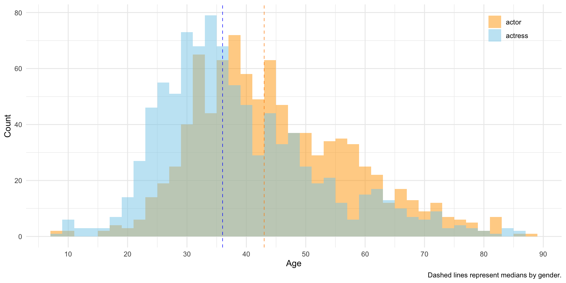
Our finding above is that for actors, but not actresses, older nominees are more likely to win than younger nominees. A side question that this raises is whether there is an age difference in nominees in the first place. The histogram below shows that there is: the typical age for women nominees is younger than men, with the most pronounced differences being the overrepresentation of women among nominees in their early 20s and the overrepresentation of men among nominees in their late 50s.
actor_median <- median(oscars$age[oscars$gender == "actor"], na.rm = TRUE)
actress_median <- median(oscars$age[oscars$gender == "actress"], na.rm = TRUE)

ggplot(oscars, aes(x = age, fill = gender)) +
  geom_histogram(position = "identity", alpha = 0.5, binwidth = 2) +
  scale_fill_manual(values = c("actor" = "orange", "actress" = "skyblue")) +
  scale_x_continuous(breaks = seq(0, 100, 10)) +
  # Add vertical lines for the medians
  geom_vline(xintercept = actor_median,
             color = "darkorange", linetype = "dashed", linewidth = .3) +
  geom_vline(xintercept = actress_median,
             color = "blue", linetype = "dashed", linewidth = .3) +
  # Add text labels for the medians
  labs(x = "Age",
       y = "Count",
       fill = NULL,
       caption = "Dashed lines represent medians by gender.") +
  theme_minimal() +
  theme(
    plot.title = element_text(hjust = 0.5, face = "bold"),
    legend.position = c(0.9, 0.9)  # Move legend to upper left corner
  )