Independence of irrelevant alternatives
A story about comedian Groucho Marx, which I first read about here is that he was in a restaurant and a waiter told him the evening’s specials were steak, fish, and chicken. Groucho ordered the steak. Somebody else at his table ordered the fish, and the waiter later came back apologetically and said that there was no fish available that evening. “In that case,” said Groucho, “I’ll have the chicken.”
The joke is that it would be irrational for Groucho’s preference for steak versus chicken to depend on whether or not fish is available. Indeed, this is a formal postulate of classical rational actor theories, known as the assumption of the independence of irrelevant alternatives (often shortened to IIA). An actor’s preference for \(A\) vs. \(B\) should not depend on whether \(C\) is available as a choice.
In the multinomial logit model, there is also an IIA assumption, so called because of its similarity to the assumption from choice theory. But it is not really the same assumption, insofar as everyone can be a perfectly rational decision maker and the IIA assumption of multinomial logit can still be violated. Instead, the issue with multinomial logit is subtler.
Intuitive example
In 2008, the Republican nominee for US President was decided much earlier than the Democratic nominee. That is, there was a period in which it was known that John McCain would be the Republican nominee, but Barack Obama and Hillary Clinton were both vying in a very close, state-by-state battle to be the Democratic nominee (Obama ended up winning the nomination and the presidency).
During this period, there were polls that asked people who they would prefer among three candidates: McCain, Obama, and Clinton. Say, for example, you use a multinomial logit to estimate the relationship between education and choice among these three candidates. The resulting coefficients for the comparison of Obama vs. McCain may be interpreted as estimating how, e.g., education is associated with a preference for Obama vs. McCain.
The problem is that, for voters who prefer Clinton, we do not observe their preference for Obama vs. McCain. Moreover, depending on what explanatory variables we have in the model, our explanatory variables may not accurately reflect how much more likely it is that Clinton voters prefer Obama to McCain.
In other words, preferences for Clinton and Obama are likely correlated with one another beyond what our observed explanatory variables indicate. And so, taking our coefficients literally would undersell the overall level of support for Obama vs. McCain, because we are underestimating how many Clinton supporters would switch to Obama if Clinton were not in the race (as would happen when Obama became the nominee.)
Violation of the IIA assumption as correlated errors of latent variables
The big picture for this section is that the above problem with Clinton and Obama can be thought of as a matter of the error terms for a person’s preferences for those candidates being correlated, when the model instead assumes they are independent. This section explains what that means in more detail, but is more technical than the rest of the page.
We have discussed how models for binary and ordered outcomes can be developed in terms of a latent continuous variable. Unordered outcomes also have a latent variable formulation, with a twist. Instead of one latent variable, there are \(k\) latent variables, where \(k\) is the number of outcome categories — though only \(k-1\) have free parameters, with the base category’s parameters constrained to 0.
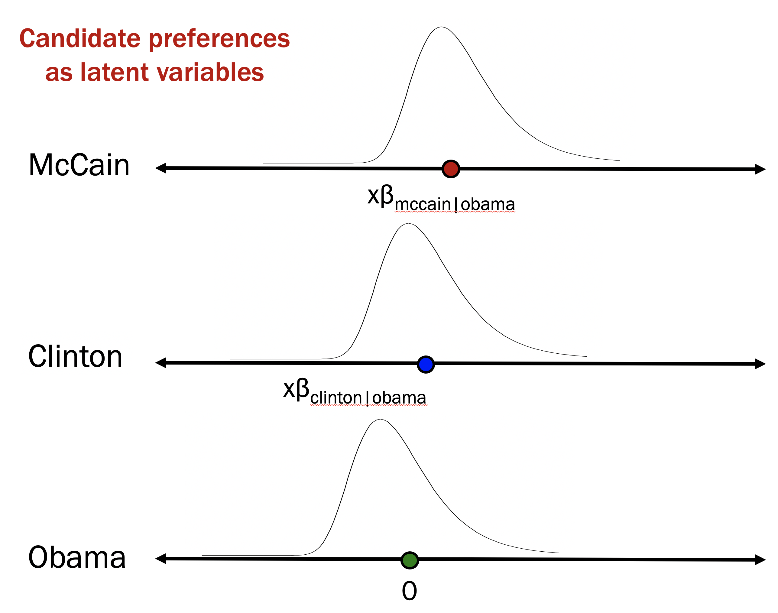
Take our example of Clinton, McCain, and Obama. We need to designate one as the base category: we will use Obama. Our three latent variables can be thought of as relating a person’s preference for each candidate to our explanatory variables and random error. We will use \(C^\ast\) to refer to the latent preference for Clinton, \(M^\ast\) for McCain, and \(O^\ast\) for Obama.
\[ \begin{align} C^\ast_i & = \mathbf{x}\beta_{C\textrm{v}O} + \varepsilon_{C,i} \\ \\ M^\ast_i & = \mathbf{x}\beta_{M \textrm{v}O} + \varepsilon_{M,i} \\ \\ O^\ast_i & = \mathbf{x}\beta_{O\textrm{v}O} + \varepsilon_{O,i} \\ \\ & = 0 + \varepsilon_{O, i} \textrm{\ (as base category)} \end{align} \]
where the candidate chosen by person \(i\) is the candidate for whom \(i\)’s preference is highest. For example, if \(M^\ast\) is greater than \(C^\ast\) and \(O^\ast\), then person \(i\) chooses McCain.
The figure below depicts an example in which, for a given set of explanatory variables, the resulting \(\mathbf{x}\mathbf{\beta}\) is highest for McCain. This means that people with that \(\mathbf{x}\) are more likely to vote for McCain than for Clinton or Obama. But, a given person with those \(\mathbf{x}\) values still has some possibility of being an Obama voter: the person’s random errors would have to be favorable enough for Obama to offset the difference \(\mathbf{x}\mathbf{\beta}\).
The IIA assumption in this formulation is then that the error terms — \(\varepsilon_{C,i}\), \(\varepsilon_{M,i}\), \(\varepsilon_{O,i}\) — are independent of one another: knowing the value of \(\varepsilon_{C}\) for person \(i\) provides no information about what \(\varepsilon_{M}\) or \(\varepsilon_{O}\) are for that person. The violation of the assumption as described above, meanwhile, is to say that \(\varepsilon_{C,i}\) and \(\varepsilon_{O,i}\) are positively correlated: if somebody has a stronger preference for Clinton than what one would predict from their explanatory variables, they also are more likely than not to have a stronger preference for Obama than one would predict from their explanatory variables.
Aside: Distribution of errors in latent variable formulation. In the figure above, the error distributions for each candidate have this unusual, asymmetric shape. This is not a mistake. For multinomial logit, the assumed error distribution is what is called a Gumbel distribution (or Type I extreme value distribution). The reason for this is pure mathematical convenience: if two random variables follow a Gumbel distribution, then the difference between them has a logistic distribution. So the Gumbel distribution is what allows the latent variable formulation above to lead to multinomial logit. (If you find this troubling, there’s also a latent variable version of the model that uses normally distributed errors, leading to a multinomial probit.)
Example
Here is General Social Survey data in which the categorical outcome is the attribute that adults think it is most important for a child to learn to prepare them for life. The options are to obey; to help others; to be well-liked; to think for oneself; and to work hard. The explanatory variables are sex, race/ethnicity (4 categories), education (3 categories), and birth year (minus 1900).
Below are the multinomial logit results, with each category in a separate column and the base category being “obey.”
------------------------------------------------------------------------------------------
                      help others     be well-liked    think for self         work hard
                             b/se              b/se              b/se              b/se
------------------------------------------------------------------------------------------
male                       -0.081             0.142            -0.271***          0.089*
                          (0.044)           (0.158)           (0.036)           (0.042)
black                      -0.919***         -0.199            -0.870***         -0.579***
                          (0.064)           (0.212)           (0.048)           (0.056)
latino                     -0.297***          0.036            -0.864***         -0.332***
                          (0.074)           (0.276)           (0.065)           (0.070)
other race/eth             -0.030             0.954**          -0.955***         -0.025
                          (0.113)           (0.301)           (0.106)           (0.108)
some col                    0.244***         -0.120             0.754***          0.330***
                          (0.055)           (0.209)           (0.044)           (0.051)
ba or above                 0.843***          0.108             1.624***          0.994***
                          (0.065)           (0.248)           (0.055)           (0.062)
birth year - 1900           0.022***         -0.004             0.015***          0.031***
                          (0.001)           (0.004)           (0.001)           (0.001)
_cons                      -1.261***         -3.200***          0.082            -1.704***
                          (0.066)           (0.209)           (0.051)           (0.066)
------------------------------------------------------------------------------------------
The highlighted coefficient is 1.624 for BA or above, with HS diploma or less as the reference category. The positive sign of this coefficient means that persons with a BA or above are relatively more likely than those with a high school degree or less to say it is most important for a child to learn to think for themselves rather than to obey.
If we exponentiate this coefficient, we could interpret it as a relative risk ratio (\(\exp(1.624) = 5.07\)). We might interpret it as:
- Compared to people with no more than a high school diploma, people with at least a college degree have over a 5 times higher relative risk of saying it is more important for a child to learn to think for themselves than to obey.
But, at least worded this way, we have smuggled in an assumption. Specifically, notice that our wording is as if everybody was asked to evaluate “think for oneself” versus “obey.” But, in fact, the only information we have for the comparison of “think for oneself” versus “obey” comes from people who rated one or the other as being the most important among the five available categories. For people who thought “help others,” “be well-liked”, or “work hard” was most important, we don’t have any information on whether they think “think for oneself” or “obey” is more important.
Instead, our estimate of \(\beta_{\textrm{think-for-oneself vs. obey}}\) is dependent only on the people who rate one or the other as most important. If we interpret this estimate as implying what we would have observed if we’d had a head-to-head comparison for everybody, then we are assuming that the logit coefficient of the head-to-head comparison by everybody is the same as what we are able to estimate from the information we have, which is just the difference among those who have one or the other category rated as most important.
How big a problem is this?
It’s straightforward that correlated errors will cause problems for predictions, such as predicting what the results from a head-to-head election between McCain and Obama would be from polls that also had Clinton as an alternative. But, often in practice, we are less interested in predictions per se than in the coefficients and the extent to which they are biased.
I have not had much luck finding published guidance about this. So I’m speaking here from a combination of my own intuitions and some simulations that support those intuitions.
Here’s my intuition, via our example of the 2008 election.
- In the Democratic primaries, Clinton did particularly well relative to Obama among White women.
- In our model, say we combined race/gender into a single variable so that we have a coefficient for white women.
- Because Clinton did well among Democrats who were White women, and McCain was of course the preference among Republican White women, the multinomial logit model coefficients for white women might look like there was an overall preference among White women for McCain vs. Obama.
- However, because preferences for Clinton and Obama were highly correlated, once Clinton dropped out of the race, Obama got support from the vast majority of White women who had been Clinton supporters.
- So, even though the multinomial logit coefficients might have suggested that Obama was less preferred than McCain among White women voters, he was in fact more preferred.
If my intuitions above are correct, then the implication is that the assumption is particularly worrisome for the coefficients of explanatory variables that distinguish between alternatives with correlated errors.
The assumption is less worrisome for coefficients that do not distinguish between the correlated alternatives but instead distinguish the correlated alternatives from the others. Someone being a Democrat, for example, did little to distinguish Obama from Clinton, even though it did a lot for McCain. And, sure, when Clinton dropped out of the race, those Clinton supporters who were Democrats overwhelmingly went for Obama, but so did Clinton supporters who were not Democrats. As a result, the Democrat coefficient for McCain vs. Obama does not change so much.
Testing the IIA assumption
There are a few different tests that have been proposed for the IIA assumption in multinomial logit. The big point, though, is that the evidence is that the performance of these tests is poor for the sorts of situations in which social scientists usually find themselves.
The most well-known test (called the Hausman or Hausman-McFadden test) does not just perform poorly, but will often give results that do not really make sense. Notably, the test is a chi-squared test, and one will often get negative test statistics, whereas chi-square values are always positive.
As a result, you are largely left on your own to decide if you consider the assumption to be violated.
Stata: Testing IIA. In the package of commands I co-authored for Stata (type \(\texttt{findit spost13\_ado}\) to download), there is one called \(\texttt{mlogtest}\) that will run a few different IIA tests. Again, I do not think these tests work well in practice.
What to do if the assumption is violated?
Proceed with the model, but recognize that your coefficients are contingent on the total set of outcome categories. This could influence your interpretation, as in changing the above statement:
- Compared to people with no more than a high school diploma, people with at least a college degree have over a 5 times higher relative risk of saying it is more important for a child to learn to think for themselves than to obey.
to something more like:
- Among the five traits provided, compared to people with no more than a high school diploma, respondents with at least a college degree had over a 5 times higher relative risk of reporting it was most important for a child to learn to think for themselves than to obey.
If the prospect of correlated errors seems really obvious and severe, one might consider turning the problem into something more like a sequential logit. For something as blatant as the McCain-Obama-Clinton example above, one might have first fit a logit for McCain vs. Obama-or-Clinton, and then fit a logit for Obama vs. Clinton. Of course, this is now making the assumption that everyone who prefers Obama-or-Clinton would pick Obama if Clinton dropped out of the race, which is also surely erroneous and hence will underestimate predicted McCain support.
One could also be in the fortunate position of having/collecting data that would give you additional leverage into the problem:
You could have ranked data. If the respondents rank their preferences for each of the categories, then you would have information for everyone on the relative preference for each outcome versus the other.
You could have alternative-specific variables as explanatory variables. These are variables that vary over the alternatives for each respondent. So, for example, in addition to a vote-preference variable for McCain vs. Clinton vs. Obama, you could have a feeling-thermometer-type measure of how the respondent feels about each candidate. In that case, there are models that elaborate on the multinomial logit that one can use to estimate the degree of dependence among different alternatives. But these models are very finicky and difficult to get estimates with ordinary survey data, so I would urge you to avoid them unless you’ve really familiarized yourself with their details and are confident with what you are doing.