In the ordered logit model, there are \(k-1\) implied binary logits, but the coefficients of each explanatory variable are assumed to be the same across all of them. This assumption is known as the parallel regressions assumption or the proportional odds assumption (the difference in these terms being that the former applies to ordered probit as well, whereas the latter only applies to logit since probit does not involve odds).
This assumption is testable.
Example
In the General Social Survey (2000-2018), subjective social class is measured in the General Social Survey with four categories: lower class, working class, middle class, and upper class. The implied binary logits are thus:
Lower vs. working, middle, and upper
Lower and working vs. middle and upper
Lower, working, and middle vs. upper
We will refer to these as U|M|W, U|M, and U, respectively, to indicate the categories constituting the \(y=1\) outcome for each of the implied binary logits.
If our explanatory variable is household income, we can imagine that these three binary logits each have different coefficients in principle: \(\beta_{inc, U|M|W}\), \(\beta_{inc, U|M}\), \(\beta_{inc, U}\).
The parallel regressions assumption is that these three regression coefficients are equal:
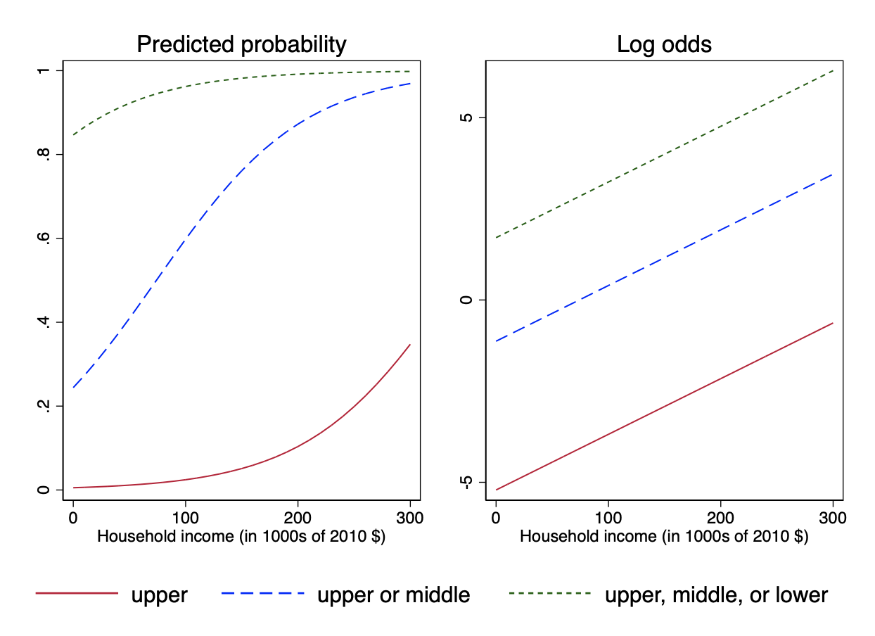
After fitting an ordered logit model, if we look at the relationship between income and the predicted probabilities – the graph on the left below – each of the curves is a fragment of a logit S-curve with the same slope, just shifted to the left or right.
But this might not be evident from the graph. If instead we look at the relationship between income and the log-odds – the graph on the right above – we can see that the different regression lines are parallel. All the differs between them is the intercept, which is what the different cutpoints determine.
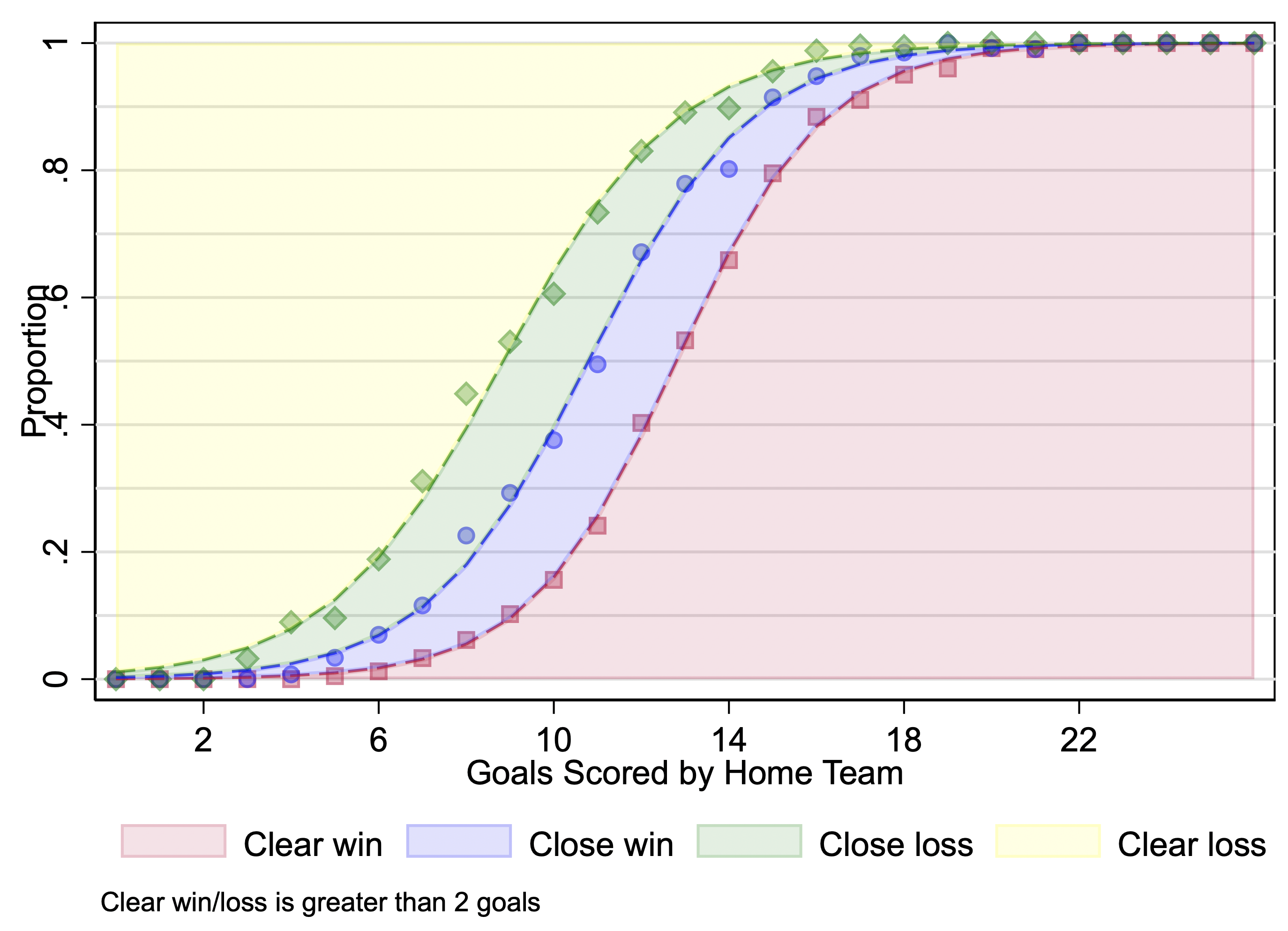
Aside: Another example of parallel regressions. Here is a graph of predicted probabilities from an ordered logit model using the data from an earlier example on women’s lacrosse games. I’m including it here because the strong relationship between goals-scored and the outcome makes it easy that the curves are parallel (that the different S-curves have the same slope and just have different intercepts; that is, they are each the same curve shifted to the left or right).
The assumption that the different regression coefficients are equal is testable. Indeed, there are a number of different ways to test it, and any of the regularly-used ones will likely do the job just fine.
One test is known as the Brant test. The basic logic of the Brant test is that it estimates the underlying implied logits, and then it computes a Wald test for the equality of coefficients. The Brant test provides both an omnibus test that is whether the coefficients for all the explanatory variables are equal across the implied binary logits, and tests for each explanatory variable on its own.
Stata: Computing the Brant test. I implemented the Brant test years ago as an add-on command in Stata, and it still works. It is the command \(\texttt{brant}\) available in the \(\texttt{spost13_ado}\) package (the command \(\texttt{findit spost13_ado}\) will include prompts to install.
We fit an ordered logit model with the explanatory variables of household income, respondent age, and survey year.
Call:
polr(formula = class ~ inc2010 + age + year, data = df, Hess = TRUE,
    method = "logistic")

Coefficients:
            Value Std. Error t value
inc2010  0.015660  1.777e-04   88.11
age      0.016740  5.064e-04   33.06
year    -0.009598  1.432e-05 -670.28

Intercepts:
                           Value       Std. Error  t value
lower class|working class     -20.3748      0.0003 -70705.2031
working class|middle class    -17.3320      0.0175   -987.8861
middle class|upper class      -13.3621      0.0353   -378.9428

Residual Deviance: 100238.20
AIC: 100250.20
. ologit class inc2010 age year, nolog

Ordered logistic regression                            Number of obs =  22,244
                                                       LR chi2(3)    = 5034.64
                                                       Prob > chi2   =  0.0000
Log likelihood = -20372.08                             Pseudo R2     =  0.1100

------------------------------------------------------------------------------
       class | Coefficient  Std. err.      z    P>|z|     [95% conf. interval]
-------------+----------------------------------------------------------------
     inc2010 |   .0153817   .0002589    59.42   0.000     .0148744    .0158891
         age |   .0173636   .0007973    21.78   0.000      .015801    .0189262
        year |   -.019298   .0022637    -8.52   0.000    -.0237349   -.0148611
-------------+----------------------------------------------------------------
       /cut1 |  -39.70182    4.54541                     -48.61066   -30.79298
       /cut2 |  -36.81336   4.544028                     -45.71949   -27.90723
       /cut3 |  -32.66689   4.543024                     -41.57106   -23.76273
------------------------------------------------------------------------------
In Stata, the Brant test may be computed using the add-on Brant command. The detail option includes the coefficients of the implied binary logits.
--------------------------------------------
Test for    X2  df  probability
--------------------------------------------
Omnibus     1654.59 6   0
inc2010     1129.62 2   0
age     346.57  2   0
year        71  2   0
--------------------------------------------

H0: Parallel Regression Assumption holds
print(brant_result)
                X2 df   probability
Omnibus 1654.58515  6  0.000000e+00
inc2010 1129.61569  2 5.094128e-246
age      346.57414  2  5.525617e-76
year      70.99767  2  3.828704e-16
. brant, detail

Estimated coefficients from binary logits

-----------------------------------------------
    Variable |  y_gt_1     y_gt_2     y_gt_3
-------------+---------------------------------
     inc2010 |    0.049      0.015      0.012
             |    32.94      46.01      32.20
         age |   -0.002      0.021      0.024
             |    -1.12      24.39       9.12
        year |   -0.039     -0.017     -0.009
             |    -8.53      -6.71      -1.29
       _cons |   78.541     31.548     11.891
             |     8.62       6.29       0.86
-----------------------------------------------
                                    Legend: b/t

Brant test of parallel regression assumption

              |       chi2     p>chi2      df
 -------------+------------------------------
          All |     858.39      0.000       6
 -------------+------------------------------
      inc2010 |     573.23      0.000       2
          age |     255.66      0.000       2
         year |      24.09      0.000       2

A significant test statistic provides evidence that the parallel
regression assumption has been violated.
The overall conclusion is that the parallel regression assumption is violated, and the results for each coefficient indicates that it violated for each coefficient.
What to do when assumption is violated?
One could fit a model that relaxes the assumptions by allowing different coefficients for the different implied logits, while still treating the outcome as ordered. The most direct version of this is known as the generalized ordered logit model.
The generalized ordered logit model is not uncontroversial, as it can produce imply predicted probabilities. (If you look at the graph above the with the log odds, imagine if the lines in that graph were not parallel. In that case, the lines could cross and crossing lines would mean that, e.g., \(\Pr(y = \textrm{middle or upper})\) is less than \(\Pr(y = \textrm{upper})\), which is impossible.)
One could fit a model for an unordered outcome, which will also have multiple coefficients for each explanatory variable. The most direct example here would be to fit a multinomial logit model.
One could fit a linear regression model, but it would be a little odd to decide this is the reason why one would fit a linear regression model, as the linear regression model would imply maybe even a stronger version of the same issue under the combination of its assumptions (1) that the relationship between the explanatory variable is linear and (2) that the distance between successive categories are unit intervals.
One could still fit the ordered logit/probit model anyway. This is guidance may not be as bad as it sounds. The Brant test could be seen as providing a stringent test for whether the ordered logit model is preferable to a solution that estimates the implied binary logits separately, especially with larger samples.
Example in which violation of assumption makes important substantive difference
In the 2000-2018 General Social Survey, I construct a 3-category measure of respondent self-described political ideology, in which 1 is “liberal” 2 is “moderate” and 3 is “conservative”. We can fit an ordered logit model looking at the relationship between this variable and educational attainment:
The reference category for the above measure of educational attainment is a high school diploma or less. As the coefficients are negative – and conservative is the highest numbered category – these coefficients could be interpreted as indicating that people with higher levels of educational attainment are less conservative.
When we do the Brant test, we can see from the implied binary logits that it is a bit more complicated than that:
library(tidyverse)library(haven)library(MASS)library(brant)# Read and prepare GSS datadf <-read_dta("../dta/gss_soc383.dta") %>%filter(as.integer(libcon3cat) <=3) %>%mutate(libcon3cat =factor(as_factor(libcon3cat)),ed3cat =as_factor(ed3cat)) %>%drop_na(ed3cat)# Fit ordered logit model with education categoriesmodel <-polr(libcon3cat ~ ed3cat,data = df, Hess =TRUE, method ="logistic")# Apply Brant test to check parallel regression assumptionbrant_result <-brant(model)
----------------------------------------------------
Test for        X2  df  probability
----------------------------------------------------
Omnibus         1297.95 2   0
ed3catsome col      157.15  1   0
ed3catba or above   1292.83 1   0
----------------------------------------------------

H0: Parallel Regression Assumption holds
print(brant_result)
                         X2 df   probability
Omnibus           1297.9514  2 1.423767e-282
ed3catsome col     157.1538  1  4.737378e-36
ed3catba or above 1292.8269  1 4.092983e-283
. brant, detail
Estimated coefficients from binary logits
------------------------------------
Variable | y_gt_1 y_gt_2
-------------+----------------------
ed3cat |
some col | -0.2420.068
| -10.17 3.06
ba or above | -0.6010.202
| -26.33 9.23
|
_cons | 1.190 -0.735
| 84.41 -57.72
------------------------------------
Legend: b/t
Brant test of parallel regression assumption
| chi2 p>chi2 df
-------------+------------------------------
All | 1297.95 0.000 2
-------------+------------------------------
2.ed3cat | 157.15 0.000 1
3.ed3cat | 1292.83 0.000 1
A significant test statistic provides evidence that the parallel
regression assumption has been violated.
From these results, we can see that the parallel regressions assumption is violated. More than this, though, when we look at the coefficients from the implied logits, we can see that, for both the indicator variables, the coefficients do not just differ across the two implied logits but are in opposite directions. What this means is that higher levels of education are associated both with being more liberal and with being more conservative. That is, college educated respondents are more likely than those without a high school diploma both to identify as liberal and to identify as conservative, because they are less likely to identify as moderate.