With subjective assessment items, like self-assessment of health or of opinion on an issue, a set of ordered categories may be easy to conceptualize as a continuum.
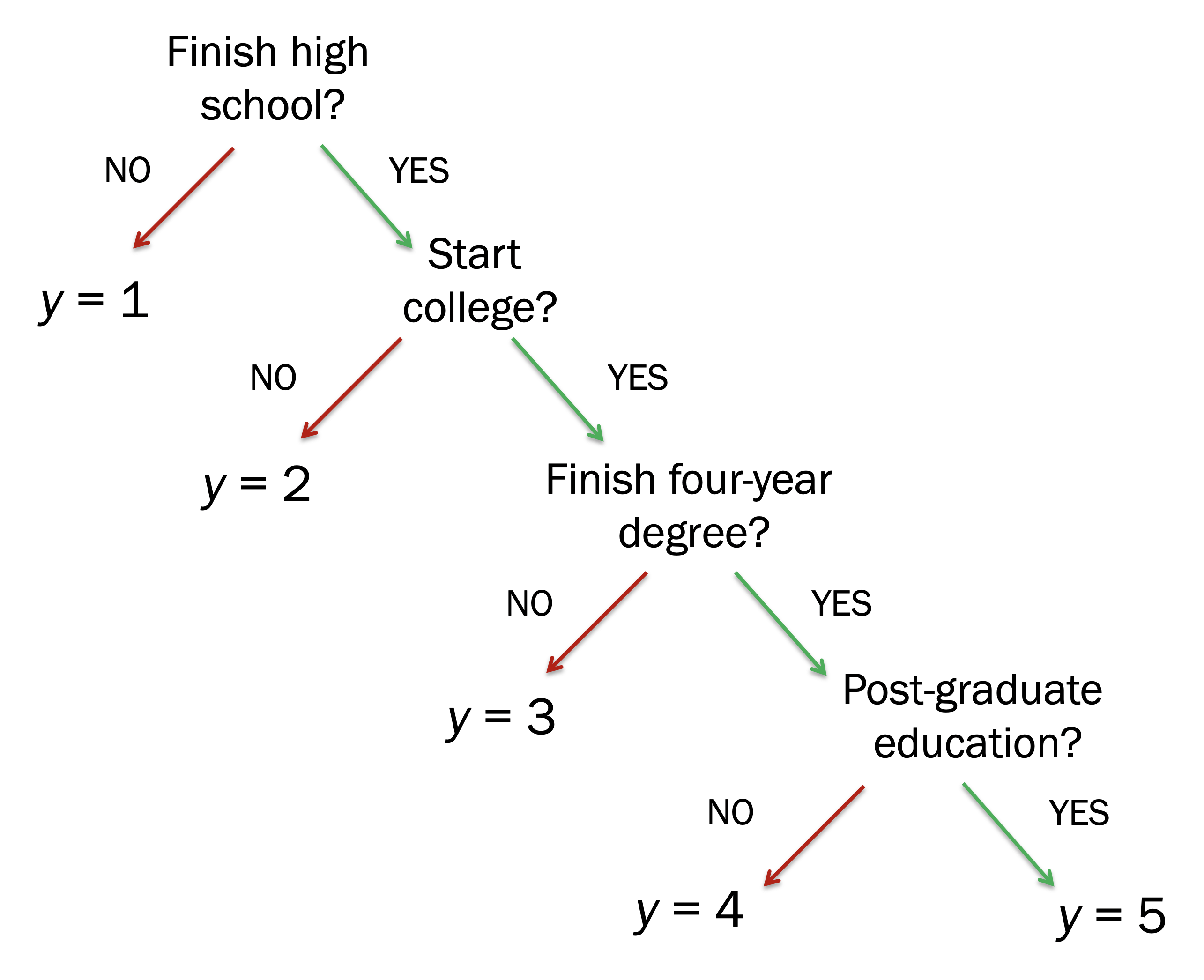
With other outcomes that also may be considered ordered, the outcome instead is more of a sequence of transitions. The example will use concerns educational attainment, and this is good for thinking about the matter. College graduates were earlier high school graduates; people with post-baccalaureate degrees were earlier college graduates. The outcome is effectively a set of stages, where higher levels of the outcome are successive stages.
Example
The data are from the National Longitudinal Study of Youth in 1979. The outcome is educational attainment, coded into five categories:
Less than a high school diploma
High school diploma but not college
Some college but not a bachelor’s level degree
Bachelor’s-level degree but no further
Post-bachelor’s level education
We will model this as a sequence of four transitions:
Does one earn high school diploma?
If one has a high school diploma, does one go to college?
If one attended college, does one earn a bachelor’s degree?
If one earned a bachelor’s degree, does one receive post-bachelor’s education?
Our explanatory variables in this example will be sex (binary), race (three categories only: White, Black, Hispanic), and mother’s education (same five categories as used for own education).
We can fit four separate logits for these four transitions. For the latter three transitions, we exclude the sample only to include those who have made the prior transition.
── Attaching core tidyverse packages ──────────────────────── tidyverse 2.0.0 ──
✔ dplyr     1.2.0     ✔ readr     2.2.0
✔ forcats   1.0.1     ✔ stringr   1.6.0
✔ ggplot2   4.0.2     ✔ tibble    3.3.1
✔ lubridate 1.9.5     ✔ tidyr     1.3.2
✔ purrr     1.2.1
── Conflicts ────────────────────────────────────────── tidyverse_conflicts() ──
✖ dplyr::filter() masks stats::filter()
✖ dplyr::lag()    masks stats::lag()
ℹ Use the conflicted package (<http://conflicted.r-lib.org/>) to force all conflicts to become errors
library(haven)library(modelsummary)# Load datadat <-read_dta("../dta/nlsy79_cda.dta") %>%drop_na(edu30, female, race, momysch) %>%filter(momysch >=0)# Create variablesdat <- dat %>%mutate(male =1- female,male =factor(male, levels =c(0, 1), labels =c("Woman", "Man")) ) %>%mutate(race =factor(race, levels =c(1, 2, 3),labels =c("White", "Black", "Hispanic")) ) %>%mutate(# Education level categorizationed_level =case_when( edu30 >=0& edu30 <=11~1, edu30 ==12~2, edu30 >=13& edu30 <=15~3, edu30 ==16~4, edu30 >=17& edu30 <=20~5 ),ed_level =factor(ed_level,levels =1:5,labels =c("No HS diploma", "HS diploma only","Some college", "BA-level college","Post-BA college")) ) %>%mutate(# Mother's educationmom_ed =case_when( momysch >=0& momysch <=11~1, momysch ==12~2, momysch >=13& momysch <=15~3, momysch ==16~4, momysch >=17& momysch <=20~5 ),mom_ed =factor(mom_ed,levels =1:5,labels =c("No HS diploma", "HS diploma only","Some college", "BA-level college","Post-BA college")) ) %>%mutate(# Sequential outcomeshsdip =ifelse(edu30 >=12, 1, 0),somecol =ifelse(edu30 >=13, 1, 0),coldeg =ifelse(edu30 >=16, 1, 0),postgrad =ifelse(edu30 >=17, 1, 0) )# Transition 1: High school diplomamod1 <-glm(hsdip ~ male + race + mom_ed, family =binomial(), data = dat)# Transition 2: Some college (conditional on HS diploma)mod2 <-glm(somecol ~ male + race + mom_ed, family =binomial(),data = dat %>%filter(hsdip ==1))# Transition 3: College degree (conditional on some college)mod3 <-glm(coldeg ~ male + race + mom_ed, family =binomial(),data = dat %>%filter(somecol ==1))# Transition 4: Post-graduate (conditional on college degree)mod4 <-glm(postgrad ~ male + race + mom_ed, family =binomial(),data = dat %>%filter(coldeg ==1))# Display resultsmodels <-list("HS dip"= mod1,"Some col"= mod2,"BA"= mod3,"Post-BA"= mod4)modelsummary(models, gof_map =c("nobs"))
Profiled confidence intervals may take longer time to compute.
  Use `ci_method="wald"` for faster computation of CIs.
HS dip
Some col
BA
Post-BA
(Intercept)
0.190
-0.702
-0.552
-0.916
(0.042)
(0.056)
(0.093)
(0.161)
maleMan
-0.317
-0.208
0.135
0.169
(0.040)
(0.048)
(0.068)
(0.099)
raceBlack
0.594
0.038
-0.787
-0.255
(0.051)
(0.058)
(0.085)
(0.142)
raceHispanic
0.416
0.260
-0.702
0.256
(0.059)
(0.073)
(0.109)
(0.177)
mom_edHS diploma only
0.711
0.823
0.555
0.065
(0.045)
(0.056)
(0.092)
(0.163)
mom_edSome college
0.976
1.859
0.932
0.367
(0.078)
(0.091)
(0.113)
(0.182)
mom_edBA-level college
1.162
2.558
1.507
0.658
(0.102)
(0.134)
(0.133)
(0.187)
mom_edPost-BA college
1.403
2.654
1.757
0.776
(0.178)
(0.220)
(0.197)
(0.233)
Num.Obs.
11862
7858
3927
1836
From this, we can see that net of other variables men are less likely to finish HS and less likely to go to college, but if they go to college, they are more likely to finish. Also we can see that, net of mother’s education, there are not significant Black-White differences for high school completion or college attendance, but Black respondents who do start college are significantly less likely to finish than their White counterparts.
------------------------------------------------------------------------------------
                              (1)             (2)             (3)             (4)
                           HS dip        Some col              BA         Post-BA
------------------------------------------------------------------------------------
#1
Man                          -.29***        -.208***         .135*           .169
                          (-4.70)         (-4.31)          (1.99)          (1.71)

Black                       -.029            .038           -.787***        -.255
                          (-0.39)          (0.66)         (-9.30)         (-1.79)

Hispanic                    -.394***          .26***        -.702***         .256
                          (-4.99)          (3.59)         (-6.46)          (1.45)

HS diploma only              1.23***         .823***         .555***         .065
                          (16.78)         (14.75)          (6.01)          (0.40)

Some college                 2.06***         1.86***         .932***         .367*
                          (11.28)         (20.39)          (8.22)          (2.01)

BA-level college             2.48***         2.56***         1.51***         .658***
                           (8.72)         (19.07)         (11.37)          (3.52)

Post-BA college              4.07***         2.65***         1.76***         .776***
                           (4.06)         (12.08)          (8.91)          (3.34)

Constant                     1.37***        -.702***        -.552***        -.916***
                          (21.38)        (-12.62)         (-5.96)         (-5.70)
------------------------------------------------------------------------------------
N                            9192            7858            3927            1836
------------------------------------------------------------------------------------
From this, we can see, for example, that net of other variables men are less likely to finish HS and less likely to go to college, but if they go to college, they are more likely to finish (note: in these data, I do not know if that is a more general phenomenon with college completion).
Also we can see that, net of mother’s education, there are not significant Black-White differences for high school completion or college attendance, but Black respondents who do start college are significantly less likely to finish than their White counterparts.
If we wanted to calculate the predicted probabilities, we would combine the probabilities from the individual logits, like so:
The add-on package \(\mathtt{seqlogit}\) allows one to estimate the separate logits of the sequential logit model as a single model. The coefficients do not change, but it easier to do some tests with everything estimated in one model.