Expand for code that loads packages
library(tidyverse)
library(haven)
library(tulaverse)
library(quantreg)We’ve seen that least squares and the mean are connected, such that the mean can be defined as minimizing the sum of squares with respect to a single variable. Or, if we use OLS to fit a model without any explanatory variables, the intercept will be the mean of the outcome. And when explanatory variables are included, linear regression estimates the conditional mean, that is, the mean holding the explanatory variable(s) to some specific value(s).
But what if we didn’t square the errors? What if we just took the absolute value of the errors instead?
If we minimize the sum of absolute deviations instead of squaring them, we get the median instead of the mean. Just as least squares provide a different way of defining the mean, absolute deviations provide a different way of defining the median. Let’s demonstrate this first.
Say we have the following set of observed values for a variable: [1, 2, 3, 9, 10]. For this set, we want to find the quantity \(c\) that minimizes the sum of absolute differences between \(c\) and each observed value.
Let’s try out some different answers for \(c\) in this case and see how well they work. We’ll start with the mean, which is 5.
For this candidate \(c\) of 5, we can calculate the sum of absolute differences \(|c - y_i|\). The first absolute difference, for example, is \(5-1=4\), since 1 is the first value in our set. The five absolute differences are \(4+3+2+4+5\), so 18 is the sum of the absolute differences.
Can we do better than that? Well, what about 4? The absolute differences when \(c=4\) are \(3+2+1+5+6=17\). 17 is less than 18, so 4 is a better answer than 5 in terms of minimizing the sum of absolute differences.
How about 3? The absolute differences when \(c=3\) are \(2+1+0+6+7=16\). 16 is less than 17, so 3 is a better answer than 4.
How about 2? The absolute differences when \(c=2\) are \(1+0+1+7+8=17\). 17 is more than 16, so 2 is a worse answer than 3.
So, 3 is the best integer answer, and 3 is also the median. But this doesn’t prove that 3 is the best answer of any possible number: what about 3.1 or 2.95? Also, just because 3 is the median in this example, this doesn’t prove that minimizing absolute deviation always results in the median.
library(tidyverse)
library(haven)
library(tulaverse)
library(quantreg)values <- c(1, 2, 3, 9, 10)
candidates <- seq(1, 10, by = 0.01)
sum_abs_diff <- sapply(candidates, function(c) sum(abs(c - values)))
df_plot <- tibble(candidate = candidates, sad = sum_abs_diff)
ggplot(df_plot, aes(x = candidate, y = sad)) +
geom_vline(xintercept = 3, linewidth = .5, color = "deepskyblue") +
geom_vline(xintercept = 5, linewidth = .5, color = "deepskyblue") +
geom_hline(yintercept = 16, linewidth = .5, color = "deepskyblue") +
geom_line(color = "red3", linewidth = 1) +
labs(x = "Candidate value", y = "Sum of absolute differences") +
theme_tula()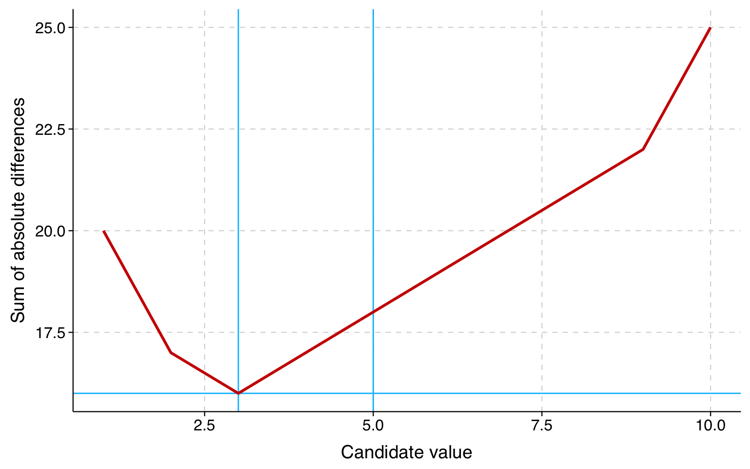
Instead, we need to understand why we arrived at the answer we did.
When we change the value of \(c\) by a tiny amount \(\delta\), the absolute difference associated with a given observation can either go up by \(\delta\), or it can go down by \(\delta\). The change \(\delta\) is the same magnitude for every observation. So whether changing \(c\) reduces the overall sum of absolute differences depends just on whether fit improves for more observations than it worsens for.
Now let’s think about the case in which \(c\) is the median. The absolute difference for the observation with the median value is 0. There are the same number of observations with values above the median as there are with values below the median.
If we increase \(c\) by a tiny amount from the median, we will fit all the observations above the median a slight bit better. But, we will fit all the observations below the median—that is, the same number of observations—a small bit worse, plus we will fit the median observation worse. So the fit worsens for more observations than it improves, and that means the sum of the absolute differences will be worse.
The same will happen if we decrease \(c\) by a tiny amount from the median. We will fit the observations below the median better, but we will fit all the observations above the median—the same number—worse, plus we will fit the median observation worse.
If we shift \(c\) from the median at all, we must and will do worse in terms of minimizing absolute differences. Therefore the median is the value that minimizes absolute differences.
We can fit a model that is the counterpart to linear regression, only instead of minimizing squared residuals, we minimize the absolute value of residuals. If we do this, our \(\mathbf{x\beta}\) estimates the conditional median instead of the conditional mean.
But let’s do this first without any explanatory variables. We will use the same data on adult heights that we did when talking about the mean.
df <- read_dta("../dta/nhanes_bodymeasures.dta") %>%
  filter(age >= 18)

summary(df$height)
Min. 1st Qu. Median Mean 3rd Qu. Max. NA's
48.54 62.99 65.75 65.89 68.74 80.51 2748 One way of obtaining the median in Stata is to use the \(\texttt{detail}\) option for the \(\texttt{summarize}\) command.
::: {.statacode}
. use ../dta/nhanes_bodymeasures, clear
(Height and weight data from NHANES adults (cumulative to 2016))

. drop if age < 18
(30,673 observations deleted)

. sum height, detail

                           height
-------------------------------------------------------------
      Percentiles      Smallest
 1%     57.40146       48.54321
 5%     59.56681       51.33848
10%     60.78728       51.81092       Obs              38,495
25%       62.992       52.16525       Sum of Wgt.      38,495

50%      65.7479                      Mean           65.88727
                        Largest       Std. Dev.      3.996099
75%     68.74002       80.23606
90%     71.18096       80.35417       Variance       15.96881
95%     72.59828       80.47228       Skewness       .1141992
99%     74.96048       80.51165       Kurtosis       2.648129
:::
The median is the value corresponding to the 50th percentile, that is, 65.7479.
In R, the function rq from the quantreg package fits a median regression model.
model <- rq(height ~ 1, data = df)
tula(model)
Median regression
Raw sum of dev = 62758.373 Number of obs = 38495
Min sum of dev = 62758.373
K-B Pseudo R2 = 0
─────────────────────────────────────────────────────────────────────────────
height │ Coef Std. Err. t P>|t| [95% Conf Interval]
─────────────────────────────────────────────────────────────────────────────
(Intercept) │ 65.75 .02789 2357 <.0001 65.69 65.8
─────────────────────────────────────────────────────────────────────────────In Stata, the command that fits a median regression model is \(\texttt{qreg}\).
::: {.statacode}
. qreg height
Iteration  1:  WLS sum of weighted deviations =  62785.795

Iteration  1: sum of abs. weighted deviations =  62785.626
Iteration  2: sum of abs. weighted deviations =  62758.373

Median regression                                   Number of obs =     38,495
  Raw sum of deviations 62758.37 (about 65.747902)
  Min sum of deviations 62758.37                    Pseudo R2     =     0.0000

------------------------------------------------------------------------------
      height |      Coef.   Std. Err.      t    P>|t|     [95% Conf. Interval]
-------------+----------------------------------------------------------------
       _cons |    65.7479   .0278948  2357.00   0.000     65.69323    65.80258
------------------------------------------------------------------------------
:::
Just like the constant term in an OLS regression model with no explanatory variables is the mean, the constant term in a median regression model with no explanatory variables is the median.
Now, let’s expand the example by computing the median separately for men and women.
tulatab(male, var=height, stat="median n", data=df)height
──────┼─────────────────
male │ Median N
──────┼─────────────────
0 │ 63.307 19,867
1 │ 68.661 18,628
──────┼─────────────────
Total │ 65.748 38,495We can use the \(\texttt{table}\) command in Stata for this.
::: {.statacode}
. table male, stat(median height)

-------------------
        |    Median
--------+----------
male    |
  0     |  63.30696
  1     |  68.66128
  Total |   65.7479
-------------------
:::
The median for males is 68.6613 and the median for females is 63.3070. The difference is thus: \(68.6613 - 63.3070 = 5.3543\).
Now we will fit a model with \(\texttt{male}\) included as an explanatory variable:
model <- rq(height ~ male, data = df)Warning in rq.fit.br(x, y, tau = tau, ...): Solution may be nonuniquetula(model)Median regression
Raw sum of dev = 62758.373 Number of obs = 38495
Min sum of dev = 45502.923
K-B Pseudo R2 = 0.275
─────────────────────────────────────────────────────────────────────────────
height │ Coef Std. Err. t P>|t| [95% Conf Interval]
─────────────────────────────────────────────────────────────────────────────
male │ 5.354 .03865 138.6 <.0001 5.279 5.43
(Intercept) │ 63.31 .02427 2609 <.0001 63.26 63.35
─────────────────────────────────────────────────────────────────────────────::: {.statacode}
. qreg height male
Iteration 1: WLS sum of weighted deviations = 45503.85
Iteration 1: sum of abs. weighted deviations = 45502.923
Iteration 2: sum of abs. weighted deviations = 45502.923
note: alternate solutions exist
Iteration 3: sum of abs. weighted deviations = 45502.923
Median regression Number of obs = 38,495
Raw sum of deviations 62758.37 (about 65.747902)
Min sum of deviations 45502.92 Pseudo R2 = 0.2750
------------------------------------------------------------------------------
height | Coef. Std. Err. t P>|t| [95% Conf. Interval]
-------------+----------------------------------------------------------------
male | 5.354317 .0382629 139.93 0.000 5.27932 5.429313
_cons | 63.30696 .026617 2378.44 0.000 63.25479 63.35913
------------------------------------------------------------------------------
:::
The conditional median for females is given by the constant term, 63.3070.
The conditional median for males is the constant term plus the coefficient for male, 63.3070 + 5.3543 = 68.6613
When presenting summary statistics, the median is sometimes preferred to the mean because it is less sensitive to extreme values. For example, official statistics on incomes and home values are often presented as medians because the extremely rich pull the mean away from the center of the distribution.
Similarly, in regression, a particular downside of minimizing squared residuals is that it means our regression coefficients are more sensitive to outliers, which can mean that our estimates might mischaracterize the vast majority of our data in order to keep from fitting outliers poorly.
As an example, we can fit OLS and median regression models on how mean/median weight changes with age among respondents aged 30-50 in NHANES.
library(modelsummary)

df_subset <- df %>%
  filter(age >= 30 & age <= 50) %>%
  drop_na(weight)

model_ols <- lm(weight ~ male + age, data = df_subset)
model_median <- rq(weight ~ male + age, data = df_subset)

modelsummary(list(model_ols, model_median),
  gof_map = c("nobs"),
output = "default")| (1) | (2) | |
|---|---|---|
| (Intercept) | 161.856 | 148.600 |
| (2.756) | (2.888) | |
| male | 24.482 | 25.969 |
| (0.819) | (0.859) | |
| age | 0.213 | 0.319 |
| (0.068) | (0.071) | |
| Num.Obs. | 12629 | 12629 |
::: {.statacode}
. quietly regress weight male age if age >= 30 & age <= 50

. estimates store ols

. quietly qreg weight male age if age >= 30 & age <= 50

. estimates store medianreg

. esttab ols medianreg, mtitles("OLS" "Median reg")

--------------------------------------------
                      (1)             (2)
                      OLS      Median reg
--------------------------------------------
male                24.48***        25.97***
                  (29.91)         (30.12)

age                 0.213**         0.319***
                   (3.14)          (4.46)

_cons               161.9***        148.6***
                  (58.73)         (51.19)
--------------------------------------------
N                   12629           12629
--------------------------------------------
t statistics in parentheses
* p<0.05, ** p<0.01, *** p<0.001
:::
In the results above, the first column is from OLS and the second from median regression.
We can interpret the two coefficients for age as follows:
In this example, the coefficients in the median regression are about 50% larger than those from OLS. It may seem counterintuitive that the median is less sensitive to outliers and yet the conditional median changes more with age.
So let’s think about this. With weight, the bigger outliers are going to be outliers in terms of extremely large, rather than small, values. Here, I show that the difference between the 1st and 50th percentile of weight is about 70 pounds, whereas the difference between the 50th and 99th percentile is over 150 pounds.
df_subset %>%
  summarize(
    p1 = quantile(weight, 0.01, na.rm = TRUE),
    p50 = quantile(weight, 0.50, na.rm = TRUE),
    p99 = quantile(weight, 0.99, na.rm = TRUE)
  )
# A tibble: 1 × 3
p1 p50 p99
<dbl> <dbl> <dbl>
1 105. 176. 333.::: {.statacode}
. summarize weight if age >= 30 & age <= 50, detail
Weight (in pounds)
-------------------------------------------------------------
Percentiles Smallest
1% 104.9 76.3
5% 119.5 77.4
10% 129.1 79.9 Obs 12,629
25% 149.2 80.7 Sum of Wgt. 12,629
50% 175.6 Mean 182.0654
Largest Std. Dev. 47.55836
75% 206.1 480
90% 241.1 480.9 Variance 2261.797
95% 269.3 490.6 Skewness 1.345123
99% 333.3 816.2 Kurtosis 8.097662
:::
Given that the slope for age is steeper in median regression than in OLS, the heaviest people in these data must be making the OLS slope flatter than it would otherwise be. To investigate, the table below shows the mean weight, median weight, and 90th percentile of weight for each age between 30 and 50.
tulatab(age, var=weight, data=subset(df, age >= 30 & age <= 50), stat="mean median p90 n")Weight (in pounds)
──────────────────────────────────────┼────────────────────────────────────
Age at Screening Adjudicated - Recode │ Mean Median P90 N
──────────────────────────────────────┼────────────────────────────────────
30 │ 177.390 169.2 238.7 631
31 │ 179.793 171.8 242.02 640
32 │ 178.803 172 235.1 623
33 │ 184.696 177.3 250.28 565
34 │ 175.006 168.7 229.1 609
35 │ 181.778 172.05 242.7 578
36 │ 180.681 170.7 243.75 616
37 │ 183.905 176.55 246.5 596
38 │ 183.6 177.5 240.96 579
39 │ 180.210 172.5 238.06 629
40 │ 185.235 177.8 253.6 667
41 │ 183.450 179.3 238.38 610
42 │ 181.322 174.7 240.08 597
43 │ 184.018 178 245.48 602
44 │ 183.177 178 237.38 617
45 │ 180.338 173.1 236.96 619
46 │ 187.354 182.4 244.65 616
47 │ 183.327 179.5 240.79 562
48 │ 182.215 174.7 239.8 526
49 │ 184.282 179.5 239.16 559
50 │ 183.526 178 236.49 588
──────────────────────────────────────┼────────────────────────────────────
Total │ 182.065 175.6 241.1 12,629::: {.statacode}
. table age if age >= 30 & age <= 50, ///
> stat(mean weight) stat(median weight) stat(p90 weight) stat(count weight)
----------------------------------------------------------------------------
| Mean Median 90th percentile Number of nonmissing values
--------+-------------------------------------------------------------------
Age |
30 | 177.3905 169.2 238.7 631
31 | 179.7925 171.8 242.1 640
32 | 178.8029 172 235.4 623
33 | 184.6958 177.3 250.4 565
34 | 175.0062 168.7 229.5 609
35 | 181.7782 172.05 242.7 578
36 | 180.6815 170.7 244.2 616
37 | 183.9045 176.55 246.6 596
38 | 183.6 177.5 241.2 579
39 | 180.2102 172.5 238.3 629
40 | 185.2351 177.8 253.9 667
41 | 183.4505 179.3 238.7 610
42 | 181.3218 174.7 240.2 597
43 | 184.0179 178 245.5 602
44 | 183.1775 178 238.7 617
45 | 180.3376 173.1 237.2 619
46 | 187.3542 182.4 246 616
47 | 183.3267 179.5 240.9 562
48 | 182.2154 174.7 239.8 526
49 | 184.2816 179.5 239.4 559
50 | 183.5262 178 237.4 588
Total | 182.0654 175.6 241.1 12,629
----------------------------------------------------------------------------
:::
Consistent with our coefficients, the median weight increases more than the mean weight across the age range.
But now look at the 90th percentile value. Whether you look at just the top or bottom rows, or scan all the numbers in that column, you’ll notice that there isn’t really an increase with age in weight at the 90th percentile. The weight of the middle respondent in each age category is increasing, but the weights of the heaviest respondents are not. As a result, since the mean is more sensitive to extreme values, the differences in the mean as age increases are less than the differences in the median.
Aside: In this example, we do not have longitudinal data, so we are not seeing individual changes in weight. Instead, age in this example cannot be distinguished from cohort, which is important here because there are ongoing cohort changes in weight: later cohorts are heavier than earlier cohorts at the same age.
Thus, for example, when we observe that the 90th percentile weights are not different for 30 year olds vs. 50 year olds in these data, that does not mean that extremely heavy people do not gain weight between ages 30 and 50. Because of the cohort trend, the extremely heavy people in this sample at age 50 were probably lighter at age 30 than the extremely heavy people in this sample are at age 30. For this reason, both the mean and the median in this example are under-estimating how much a person’s weight changes with age, because the increase in a person’s weight with age is partially offset by earlier cohorts being lighter (at the same age) than later cohorts.
Median regression is just a special, simplest case of a broader class of models known as quantile regression. Quantile regression estimates a specific quantile of the outcome conditional on explanatory variables; median regression is the special case for the 50th percentile.
Stata: Quantile regression. The command that estimates median regression is called \(\texttt{qreg}\) because that is short for quantile regression. \(\texttt{qreg}\) fits median regression by default, but if you want to fit some other percentile, you add the option \(\texttt{q(}\textrm{#}\texttt{)}\), where # is the fraction corresponding to the quantile you want. That is, option \(\texttt{q(.5)}\) is median regression.
Above, we looked at descriptive statistics and showed that there didn’t seem to be much of a relationship between age and weight for those in the 90th percentile of weight.
model_q90 <- rq(weight ~ age + male, data = df_subset, tau = 0.9)
tula(model_q90)
90th Quantile regression
Raw sum of dev = 125744.600 Number of obs = 12629
Min sum of dev = 124139.603
K-B Pseudo R2 = 0.01276
─────────────────────────────────────────────────────────────────────────────
weight │ Coef Std. Err. t P>|t| [95% Conf Interval]
─────────────────────────────────────────────────────────────────────────────
age │ -.1083 .1796 -.6031 .5464 -.4604 .2437
male │ 20.38 2.16 9.432 <.0001 16.14 24.61
(Intercept) │ 234.8 7.508 31.27 <.0001 220.1 249.5
─────────────────────────────────────────────────────────────────────────────::: {.statacode}
. qreg weight age male if age >= 30 & age <= 50, q(.9) nolog
.9 Quantile regression Number of obs = 12,629
Raw sum of deviations 125744.6 (about 241.10001)
Min sum of deviations 124139.6 Pseudo R2 = 0.0128
------------------------------------------------------------------------------
weight | Coef. Std. Err. t P>|t| [95% Conf. Interval]
-------------+----------------------------------------------------------------
age | -.1083336 .1806909 -0.60 0.549 -.4625153 .2458481
male | 20.37501 2.178437 9.35 0.000 16.10494 24.64508
_cons | 234.775 7.334634 32.01 0.000 220.398 249.152
------------------------------------------------------------------------------
:::
The coefficient for age here is negative—opposite in sign from our models above—and not statistically significant. The results from our quantile regression are thus right in line with what we observed looking at the 90th percentile of weight by age.
R: Quantile regression. To fit a quantile regression in R, one may use the \(\texttt{rq()}\) function provided as part of the \(\texttt{quantreg}\) package. When doing so the argument \(\texttt{tau = .5}\) indicates median regression, whereas other values of \(\texttt{tau}\) estimate coefficients for other quantiles.
Key points