Click for code to load packages
library(tidyverse)
library(haven)
library(tulaverse)Somewhere along the way you learned that what is usually called an average is more technically termed a mean. If I asked you what a mean is, you would probably answer by providing the recipe for how one goes about computing it:
\[ \text{mean} = \frac {\text{sum of all values}}{\text{number of observations}} \]
that is:
\[ \text{mean}(x) = \frac {\sum_{i=1}^{N} x_i} {N} \]
Notice that this way of defining a mean, while correct, does not really get at why the mean is a measure of center of a distribution, nor by what criterion a mean might be asserted to provide a better measure of center than any other number.
As a result, this usual way of thinking about a mean doesn’t really go anywhere, even though we know that the mean is fundamentally connected to other quantities that are important in social statistics, like the standard deviation or the predicted values from regression.
On the other hand, when learning regression analysis, one is introduced to a criterion: least squares. It is the LS in OLS regression. That OLS minimizes the sum of squared errors is not some incidental math fact, but its defining feature.
As it turns out, least squares and the mean are fundamentally related. Here we will see how!
Consider a simple example with the values \([1, 2, 3, 9, 10]\). We can easily calculate the mean: \[ \frac {1+2+3+9+10} {5} = \frac {25} {5} = 5 \]
Now, let’s consider least squares for this same set of values. We are used to thinking about least squares of an outcome variable when regressed on explanatory variables, but we do not actually need an explanatory variable to have a least squares estimate.
For a given set of values \(y_i\), we want to find the value \(c\) that minimizes the sum of squared distances between \(y_i\) and \(c\).
A brute-force way we can solve for \(c\) is by trying a bunch of candidate possibilities for \(c\), computing the sum of squared errors for each, and seeing which performs the best. This is what we did before.
In the graph below, the x-axis shows different candidate values of \(c\). The y-axis values are the sums of squared errors:
\[\sum_{i=1}^{5}(y_i - c)^2\]
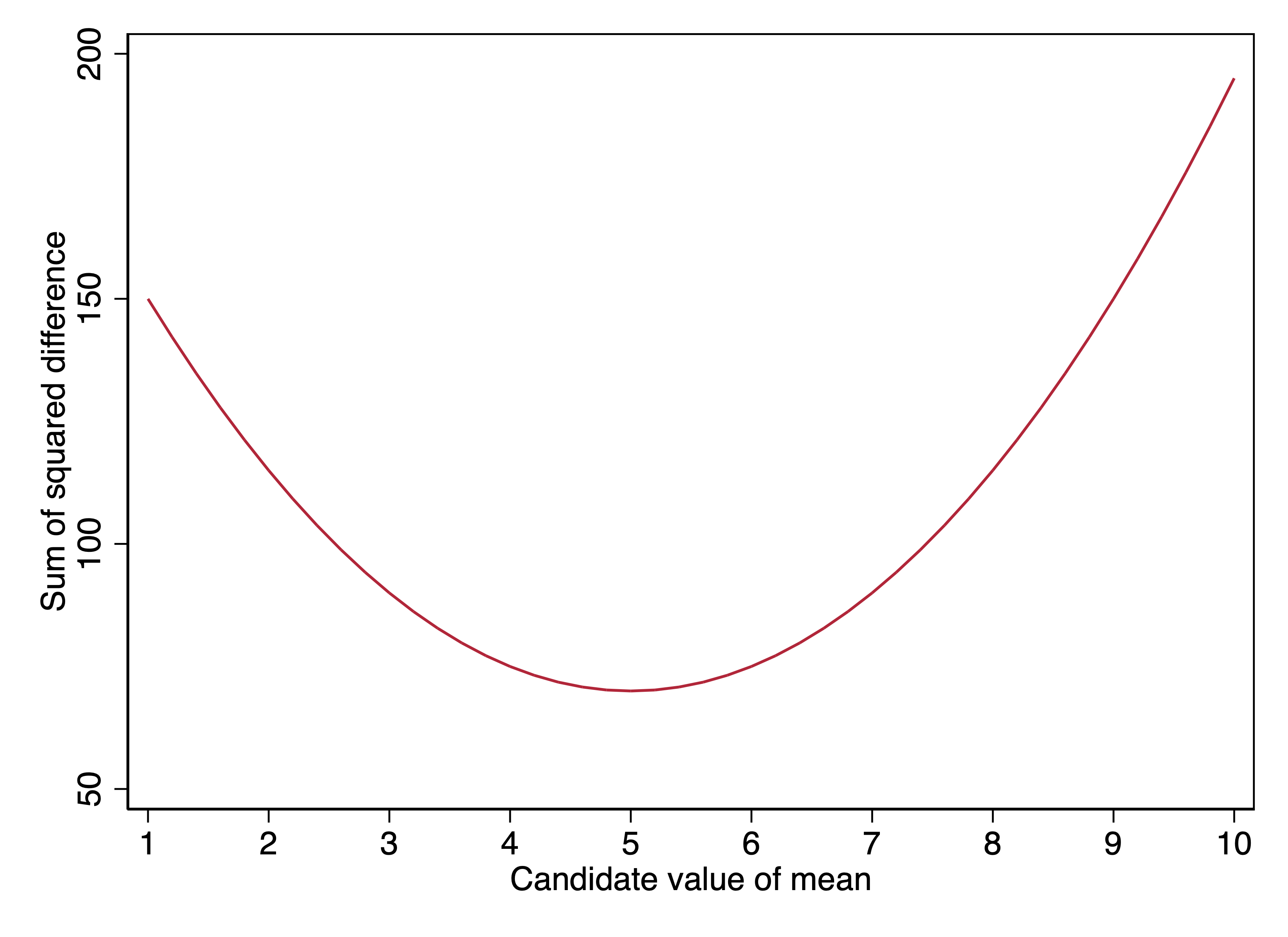
We see that the lowest sum of squared errors is at \(c=5\), that is, when the candidate value of \(c\) is the mean. For a single variable, the value that minimizes the sum of squared errors between that value and the values of the variable is the mean.
Of course, this single example doesn’t prove that assertion. But I can prove it! Multiple ways! I do so for the interested reader below.
You can also see this empirically with any variable in any dataset of your choosing. For example, here is NHANES data on the height of adults. In Stata, we can use the \(\texttt{summarize}\) command to get the mean height for the sample:
. use ../dta/nhanes_bodymeasures, clear
(Height and weight data from NHANES adults (cumulative to 2016))

. drop if age < 18
(30,673 observations deleted)

. sum height

    Variable |        Obs        Mean    Std. Dev.       Min        Max
-------------+---------------------------------------------------------
      height |     38,495    65.88727    3.996099   48.54321   80.51165
library(tidyverse)
library(haven)
library(tulaverse)
df <- read_dta("../dta/nhanes_bodymeasures.dta") %>%
filter(age >= 18)
tula(height, data=df) # summary statistics for variable──────────────────────────────────────────────────────────────────
Variable │ Obs Mean Std. dev. Min Max
──────────────────────────────────────────────────────────────────
height │ 38495 65.887 3.996 48.543 80.512
──────────────────────────────────────────────────────────────────The mean is 65.89 inches. Now, let’s fit an OLS regression without any explanatory variables:
::: {.statacode}
. regress height

      Source |       SS           df       MS      Number of obs   =    38,495
-------------+----------------------------------   F(0, 38494)     =      0.00
       Model |           0         0           .   Prob > F        =         .
    Residual |  614703.342    38,494  15.9688092   R-squared       =    0.0000
-------------+----------------------------------   Adj R-squared   =    0.0000
       Total |  614703.342    38,494  15.9688092   Root MSE        =    3.9961

------------------------------------------------------------------------------
      height |      Coef.   Std. Err.      t    P>|t|     [95% Conf. Interval]
-------------+----------------------------------------------------------------
       _cons |   65.88727   .0203673  3234.95   0.000     65.84735    65.92719
------------------------------------------------------------------------------
:::
model <- lm(height ~ 1, data = df)
tula(model)
AIC = 215902.764 Number of obs = 38495
BIC = 215919.881 R-squared = 0
Adj R-squared = 0
Root MSE = 3.996
─────────────────────────────────────────────────────────────────────────────
height │ Coef Std. Err. t P>|t| [95% Conf Interval]
─────────────────────────────────────────────────────────────────────────────
(Intercept) │ 65.89 .02037 3235 <.0001 65.85 65.93
─────────────────────────────────────────────────────────────────────────────The estimate for the constant is exactly the same: the mean.
We know that OLS regression minimizes the sum of \((\hat{y}_i - y_i)^2\). In this case, because there are no explanatory variables in the model, \(\hat{y}_i\) is the same for every observation: 65.89, or the mean. If there are no explanatory variables in a model, the predicted value of \(y\) that minimizes the sum of squared errors is the mean of \(y\). This is another way of pointing out that the mean minimizes squared errors.
A conditional mean is a mean specific to observations that share the same value(s) of the explanatory variable(s). Using the height data from NHANES, we can compute conditional means by sex: that is, the mean for women and the mean for men.
::: {.statacode}
. table male, c(mean height)

------------------------
     male | mean(height)
----------+-------------
   female |     63.29311
     male |     68.65397
------------------------
:::
df %>%
  group_by(male) %>%
  summarize(mean_height = mean(height, na.rm = TRUE))
# A tibble: 2 × 2
male mean_height
<dbl> <dbl>
1 0 63.3
2 1 68.7We can see in this table that the mean height for women in NHANES is 63.3 inches and the mean height for men is 68.7 inches. These are conditional means (specifically, they are means conditional on respondent sex).
As we saw above, if one fits an OLS regression with no explanatory variables, the constant (\(\beta_0\)) is the overall mean of the outcome. When we do add explanatory variables, OLS is a model of the conditional mean.
By this, I mean that \(\hat{y_i}\) in OLS estimates the mean of \(y\) conditional on the value(s) of \(x\) for observation \(i\).
If we fit a regression model in which
\[\hat{\text{height}}_i = \beta_0 + \beta_1(\text{male}_i)\]
Then the conditional mean for women is:
\[ \begin{align} \hat{\text{height}}_i & = \beta_0 + \beta_1(\text{0}) \\ & = \beta\_0 \end{align} \]
And the conditional mean for men is:
\[ \begin{align} \hat{\text{height}}_i & = \beta_0 + \beta_1(\text{1}) \\ & = \beta_0 + \beta_1 \end{align} \]
If we fit the regression model:
::: {.statacode}
. regress height male

      Source |       SS           df       MS      Number of obs   =    38,495
-------------+----------------------------------   F(1, 38493)     =  31426.28
       Model |  276287.741         1  276287.741   Prob > F        =    0.0000
    Residual |  338415.601    38,493  8.79161409   R-squared       =    0.4495
-------------+----------------------------------   Adj R-squared   =    0.4495
       Total |  614703.342    38,494  15.9688092   Root MSE        =    2.9651

------------------------------------------------------------------------------
      height |      Coef.   Std. Err.      t    P>|t|     [95% Conf. Interval]
-------------+----------------------------------------------------------------
        male |   5.360851   .0302404   177.27   0.000     5.301579    5.420123
       _cons |   63.29312   .0210362  3008.77   0.000     63.25188    63.33435
------------------------------------------------------------------------------
:::
model <- lm(height ~ male, data = df)
tula(model)
AIC = 192928.444 Number of obs = 38495
BIC = 192954.119 R-squared = 0.4495
Adj R-squared = 0.4495
Root MSE = 2.965
─────────────────────────────────────────────────────────────────────────────
height │ Coef Std. Err. t P>|t| [95% Conf Interval]
─────────────────────────────────────────────────────────────────────────────
male │ 5.361 .03024 177.3 <.0001 5.302 5.42
(Intercept) │ 63.29 .02104 3009 <.0001 63.25 63.33
─────────────────────────────────────────────────────────────────────────────Our results are that:
\[\hat{\text{height}}_i = 63.29 + 5.36(\text{male}_i)\]
The example is simple because sex is measured as a binary variable and is the only explanatory variable in our model. Thus the sample can be divided into two groups, and calculating the mean for each group is straightforward.
Once we have models with multiple explanatory variables, including some which are continuous, we quickly get into the situation where many observations have configurations of explanatory variables that are unique within that sample. In other words, if our set of explanatory variables are sex, age, race/ethnicity, education, and household income, we may have many observations that are unique in our sample in terms of their particular combination of these five variables. Nevertheless, the same logic applies: \(\hat{y}_i\) is our best estimate of the conditional mean for observations sharing observation \(i\)’s values of the explanatory variables.
Key points
Supplement: Proof that the mean minimizes the sum of squared distances
We want to find the value of \(c\) that minimizes \[\sum_{i=1}^{N}\left[(y_i - c)^2\right]\] that is, the squared distances between \(y_i\) and \(c\). By definition, that value will be our least squares estimate.
Trying to find the value that minimizes a function is one of the tasks for which calculus was invented.
Specifically, in the case of \[\sum_{i=1}^{N}\left[(y_i - c)^2\right]\], we have a function that will minimize at a single point, with a negatively sloped line to the left of that minimum and a positively sloped line to the right of that minimum. So finding the value at which the function is minimized is the same as finding the only value at which the slope of the function is 0.
We want to find the value of \(c\) at which the derivative of \(\sum_{i=1}^{N}\left[(y_i - c)^2\right]\) is 0.
The derivative of \(\sum_{i=1}^{N}\left[(y_i - c)^2\right]\) is proportional to: \[\sum_{i=1}^{N}\left[(c - y_i)\right]\]
In other words, if we find the value of \(c\) for which the sum of the distances \(\left[(c - y_i)\right]\) is 0, we find the value of c that minimizes the sum of the squared distances.
So now we need to solve for \(c\):
\[\sum_{i=1}^{N}\left[(y_i - c)\right] = 0 \]
\[\sum_{i=1}^{N}y_i - \sum_{i=1}^{N}c = 0 \]
\[\sum_{i=1}^{N}y_i = \sum_{i=1}^{N}c \]
Since \(c\) is a constant, the sum of \(c\) from 1 to \(N\) is \(c \times N\), meaning that:
\[\sum_{i=1}^{N}y_i = c N \]
\[\frac{\sum_{i=1}^{N}y_i}{N} = c \]
where \(\frac{\sum_{i=1}^{N}y_i}{N}\) is the sum of all observations over the number of observations–that is, the mean.