We are going to first appeal to your intuit with a simple, hypothetical scenario. Say you are starting to field a large survey on a random sample of folks and you want an accurate estimate of how long it will take.
You have two different estimates of survey length provided by two different sources.
Both estimates agree that survey length will be normally distributed with a standard deviation of 3 minutes.
Estimate A is that the mean survey length will be 15 minutes.
Estimate B is that the mean survey length will be 20 minutes.
The first three surveys come in and their lengths are 18, 20, and 21 minutes.
Given this information, either of these estimates might be correct, in the sense of reflecting the average length you will observe after fielding a very large number of surveys.
However, if Estimate A is correct, though, it’s very fluky that we would have the first three surveys all be so far off the mean. If Estimate B is correct, meanwhile, it’s not so fluky that we’d have observed the lengths for the first three surveys that we did.
My hope is that you agree that, given the evidence we have so far, Estimate B appears to be a better estimate than Estimate A. For example, if we had to choose one estimate or another for the purpose of any decision-making, we would go with Estimate B, even though ultimately it could be that Estimate A is actually correct. If you do agree with this, congratulations! You have taken the first step toward understanding maximum likelihood estimation!
The basic idea here is that the three survey lengths that we observed are more likely (less fluky) in a world in which Estimate B was correct rather they are in a world in which Estimate A is correct. And for that reason, we prefer Estimate B.
The way this toy example connects to maximum likelihood regression models is that, instead of Estimate A and Estimate B, in regression models we have a space of possible estimates of our model parameters (e.g., our \(\beta\) coefficients). We need a way of adjudicating among these possible estimates to decide which are our preferred estimates given the data we have. OLS does this in linear regression by minimizing the sum of squared errors. Maximum likelihood estimation has broader applicability than OLS–even though it gives the same answers in the specific case of linear regression–and it is based on the same principle as our toy example.
In maximum likleihood estimation, a set of estimates is considered best because, if those estimates were correct, the data we observed are least fluky.
Toy example, continued
Above, we just made a qualitative judgment that our observed survey lengths are more likely under Estimate B than Estimate A. In fact, we can precise about this. It’s all about the normal curve.
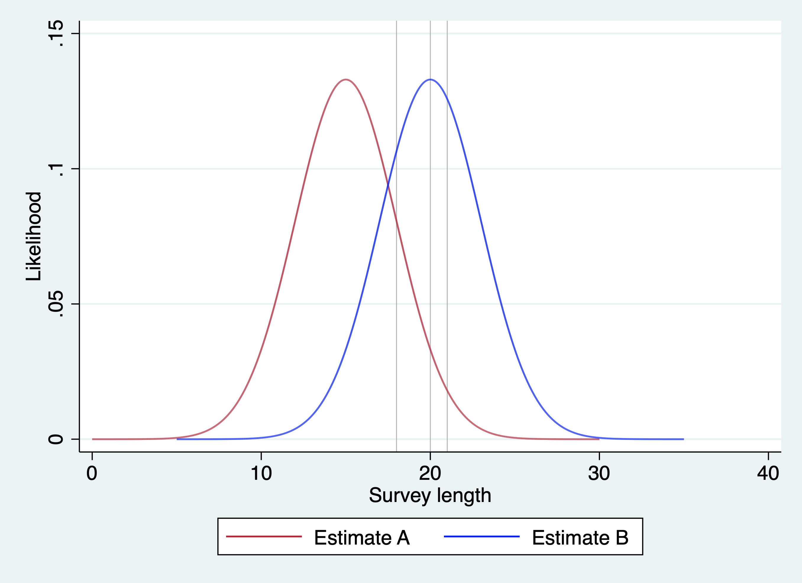
In this graph, the red and blue lines represent the distribution of survey lengths implied by Estimate A (red) and Estimate B (blue). The gray vertical lines represent the lengths of the three surveys we observed.
Notice that the gray lines in this example always intersect Estimate B at a higher point on the y-axis than Estimate A. That means that for each of the three surveys, the observed length was more likely if Estimate B is correct than if Estimate A is correct.
We can be even more precise than this. The values on the y-axis indicate the likelihood of observing a given survey length, if the estimate is correct. That is, the likelihood is the y-axis value at the point where the normal curve for an estimate intersects the gray line representing an observation.
I do not want to get into the math of computing these likelihood values here, because the point is to build intuition. So I am just going to list what these likelihoods are here:
For Estimate A, the likelihoods for the three observations are: [.0806, .0330, .0180]. If we multiply these together, we get .00005054.
For Estimate B, the values of the y-axis that intersect the three observations are: [.1062, .1330, .1259]. If we multiply these together, we get .001778.
Sure, .001778 might be a small number, but it is more than 35 times larger than .00005054. For our purposes, this means that the survey lengths that we observed are about 35 times more likely to happen in a world in which Estimate B are the correct estimate than Estimate A.
Log-likelihoods instead of likelihoods
If you have followed the example to this point, you’ve already got the most important point of it. For that reason I hate to throw this in, and so I wouldn’t if it so wasn’t important. When I combined the likelihoods above, I did so by multiplying them together.
I multiplied them together for the same reason that when you want the combined probability of a set of independent events, you multiply the probability of each event together. For example, the probability of rolling two 1s on a pair of dice is \((\frac{1}{6})(\frac{1}{6})=(\frac{1}{36})\) because the probability of rolling a 1 on one die is 1/6 and so you multiply 1/6 by 1/6 to get the combined probability.
In our above example, instead of multiplying the likelihoods, we could have logged them first and then just added them up.
For Estimate A, the log-likelihoods are: -2.5175, -3.4120, -4.0175, and their sum is -9.9471.
For Estimate B, the log-likelihoods are: -2.2420, -2.2018, -2.0720, and their sum is -6.5158.
The difference is 3.413, and if we exponentiate that difference: \(\exp(3.413) \approx 35\). (The difference with the prior result is just due to rounding along the way.) The big point is that we ultimately would have gotten the same result by adding together log-likelihoods that we got by multiplying likelihoods.
Why do this? It might not seem like logging a set of numbers and then adding them together is easier than multiplying them. But for the computer it is. Especially when we start talking about doing this over thousands or tens of thousands or millions of observations. The log approach then is much, much quicker and easier for a computer to handle than keeping track of all the zeros for a product that keeps getting smaller and smaller.
For this reason, when we do maximum likelihood estimation, in practice the work is with log-likelihoods rather than likelihoods. As a result, in output and elsewhere, you will see results in terms of log-likelihoods rather than likelihoods.
Log-likelihoods and linear regression
We discussed least squares earlier via an example of data in which the outcome was how much money a movie made and the explanatory variable was its Rotten Tomatoes score. Let’s revisit that example.
As before, we have centered both the explanatory variable and the outcome, so that we do not have to worry about estimating the intercept. The only parameter is \(\beta_{RT}\), the coefficient for the Rotten Tomatoes score.
Let’s consider two scenarios:
Estimate A: \(\beta_{RT}\) is .5
Estimate B: \(\beta_{RT}\) is 1
Let’s consider an example of one of the movies in the dataset, We Bought a Zoo.
We Bought a Zoo had a Rotten Tomatoes score that was 18.8 points above the mean. As a result, Estimate A would predict the movie to have made 9.4 million dollars more than the mean, while Estimate B would predict the movie would gross 18.8 more than the mean. Alas, We Bought a Zoo actually made less 19.5 million dollars less than the mean.
In this case, Estimate A fits better than Estimate B. While we won’t do the math of converting this to a likelihood, the likelihood of the errors is about .396 for Estimate A and .387 for Estimates B. So it is only a little bit more likely that we would have observed the error we did if Estimate A was correct than if Estimate B (it works out to about 2%).
The output above shows the log-likelihoods as well. Because the likelihoods are \(< 1\), the log-likelihoods are negative. So don’t be fooled: Estimate A’s log-likelihood is greater than Estimate B’s, because it is closer to 0.
Where Estimate B more than makes up for these sorts of differences is in the cases that end up having really large errors in this model because they are films that make much more than one would predict (in this case, making way more money than one would predict regardless of its RT score).
The movie Avatar is the biggest case in point. Avatar had the biggest US gross of all time.
Avatar made $684M more than the mean movie, so even Estimate B’s larger prediction of $35.8M above the mean seems way off. But, as we discussed, least squares hates outliers and will give big rewards even for modest improvement in fitting extreme observations.
We can see this when we look at the likelihood and log-likelihoods:
# Calculate sum of log-likelihoods for all observationsdf %>%summarise(sum_ln_likelihood_a =sum(ln_likelihood_a, na.rm =TRUE),sum_ln_likelihood_b =sum(ln_likelihood_b, na.rm =TRUE) )
First, notice how small these likelihoods are. 3.66e-17 means .0000000000000000366. And this is just one observation. This is why it is easier for the computer to work with log-likelihoods. These numbers get really small and then the computer not only has to keep track of the 3.66 part but all the 0’s in front of it.
Compare the difference in log-likelihoods here to that for We Bought a Zoo. For We Bought a Zoo, the log-likelihood difference between the two estimates was about .02 in favor of Estimate A. For Avatar, the log-likelihood difference is about 2. This works out to the error for Estimate B being more than 7 times more likely (that is, 800%).
Over all the 609 movies, the sum of the log-likelihoods ends up being -875.65 for Estimates A and -863.54 for Estimates B. Estimates B has the greater log-likelihood, and so we would prefer it.
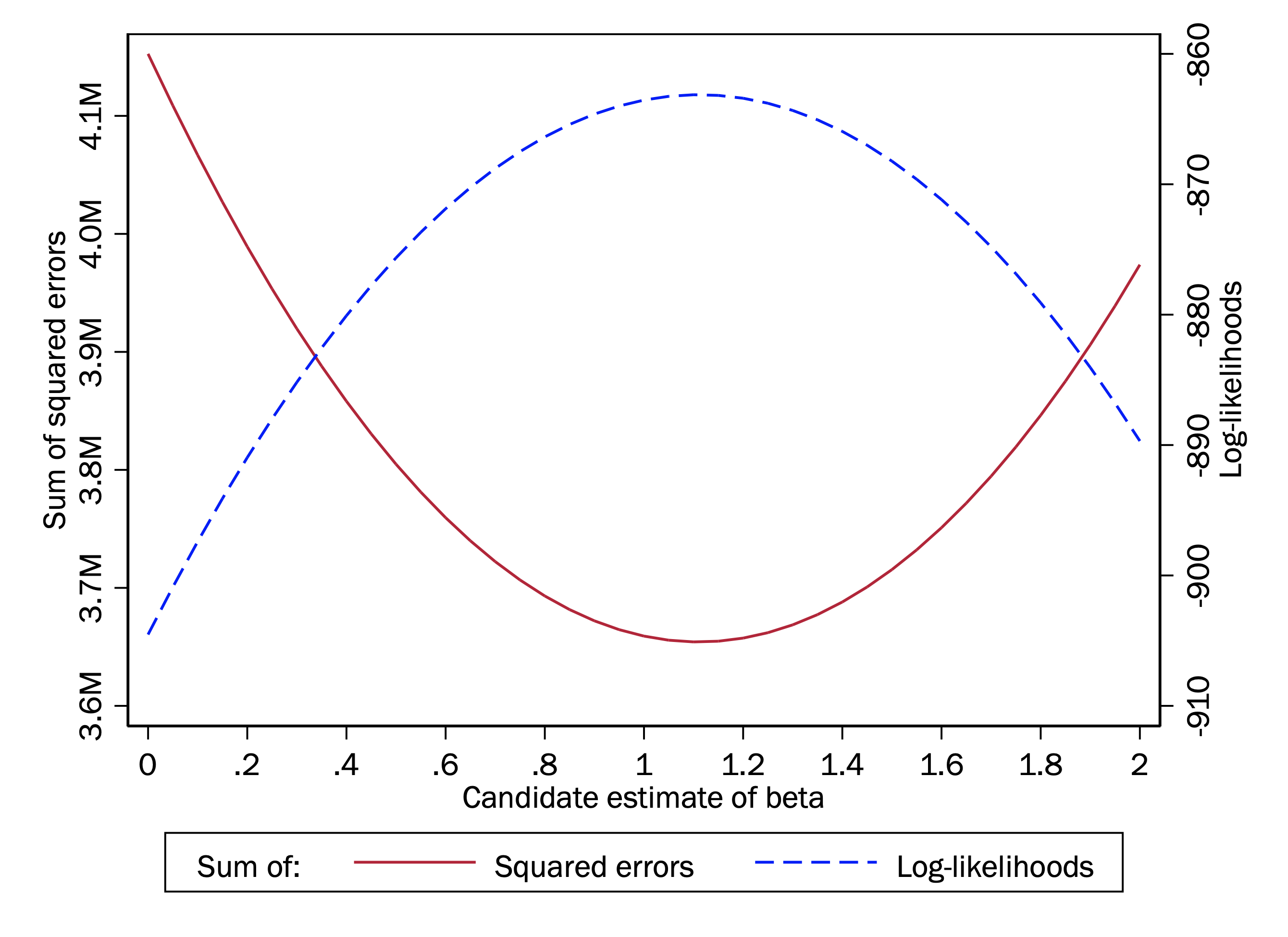
As we did before with least squares, we can try a whole range of estimates, and evaluate their log-likelihood. Indeed, we can plot this on the same graph as the sum of squares.
As you can see, the two functions here have the same shape, except one the inverse of the other. And the scales differ. But the value of \(\beta\) that minimizes the sum of squares is exactly the same as the one that maximizes the log-likelihood.
Say we have two potential sets of estimates for our coefficients, which we will call \(\hat{\mathbf{\beta}^A}\) and \(\hat{\mathbf{\beta}^B}\). Which do we consider better? With least squares, the better \(\hat{\mathbf{\beta}}\) is the one that minimizes the sum of squared errors. That fact does not provide a very strong conceptual foundation for thinking about why we these estimates are preferred, and it doesn’t provide something we can build off for thinking about what we should do when least squares is not an available approach.
Stating the big idea again
For the linear model, we can get to the same result as least squares with a different approach, using what we have just shown regarding the normal distribution and the likelihood of observing errors of a given size.
Some estimates, in other words, imply that the values of the outcomes that we observed are far more unlikely than they are given other estimates.
Say your outcome is height. If you have a sample of 500 and a set of estimates that misses everybody’s height by five inches, it is possible that those estimates are still the correct estimates of the population parameters. But it is extremely unlikely that you’d have observed the heights that you did if that was the case. If you had a different set of estimates that missed everybody’s height by two inches, the heights we observed wouldn’t be as unlikely.
This is the core idea of maximum likelihood estimation. You have some data and some unknown parameters that you want to estimate. You have a whole space of estimates that are possibly the population parameters, but you want to choose which ones are best. With maximum likelihood estimation, one looks at a set of possible estimates and asks, “If these were the true population parameters, how likely is it we would have observed the values of the outcome that we observed for each of these observations, given their values of the explanatory variables?”
In truth, the answer for every possible estimate is going to be extremely unlikely, because we are talking about the likelihood of observing exactly the configuration of outcome values that we observed. But just because everything is extremely unlikely doesn’t mean that some estimates imply our data are even more wildly unlikely than others. And what we want are the estimates that make the outcome values we observed least unlikely–that is, most likely. Maximum likelihood gives us a reason to select one set of \(\hat{\mathbf{\beta}}\) over all the others: we select the \(\hat{\mathbf{\beta}}\) that imply the highest likelihood of observing the values of the outcome that we actually observed.
Key points
What we are doing here is taking a first pass at the idea of maximum likelihood estimation.
The big idea of maximum likelihood estimation is that the criterion we use for deciding which estimates are best is which estimates imply that the outcomes we observed are most likely (that is, least fluky)
Because it is much easier for software to work with (and some other reasons), in practice when we maximize likelihood what we are really doing is maximizing the sum of log-likelihoods. This is just a transformation that makes no difference whatsoever for our estimates.