There are two important drawbacks to the linear probability model.
Problem #1: The LPM can produce impossible predictions
Probabilities can never be less than 0 or greater than 1. Yet, in the linear probability model, there is nothing that constrains predicted probabilities to the range between 0 and 1.
In the model, the relationship between \(x\) and the predicted probability is linear, and there is nothing stopping that line from going above 1 or below 0 for the more extreme values of \(\mathbf{x}\). Indeed, unless the coefficient for \(x\) is exactly zero, there will always be values of \(x\) for which predicted probabilities fall outside this range; the only question is whether those values of \(x\) are plausible or not.
For example, here is some data from the 1970s in which the outcome is labor force participation in a sample of US women. The variable \(\texttt{k5}\) is the number of children under the age of 6, and \(\texttt{k618}\) is number of children ages 6-18.
The constant term is .609—the predicted probability of being in the labor force for a woman with no children. Meanwhile, the coefficient for k5 implies that each child under age 6 decreases this predicted probability of labor force participation by .203.
If a woman has three children under the age of 6 (and no kids aged 6-18), her predicted probability of being in the labor force is -.001. If she has 4 kids under the age of 6, her predicted probability is -.20.
While having 3 or 4 children under the age of 6 is unusual, it is hardly unheard of.
My own mom was an example at one point in her life.
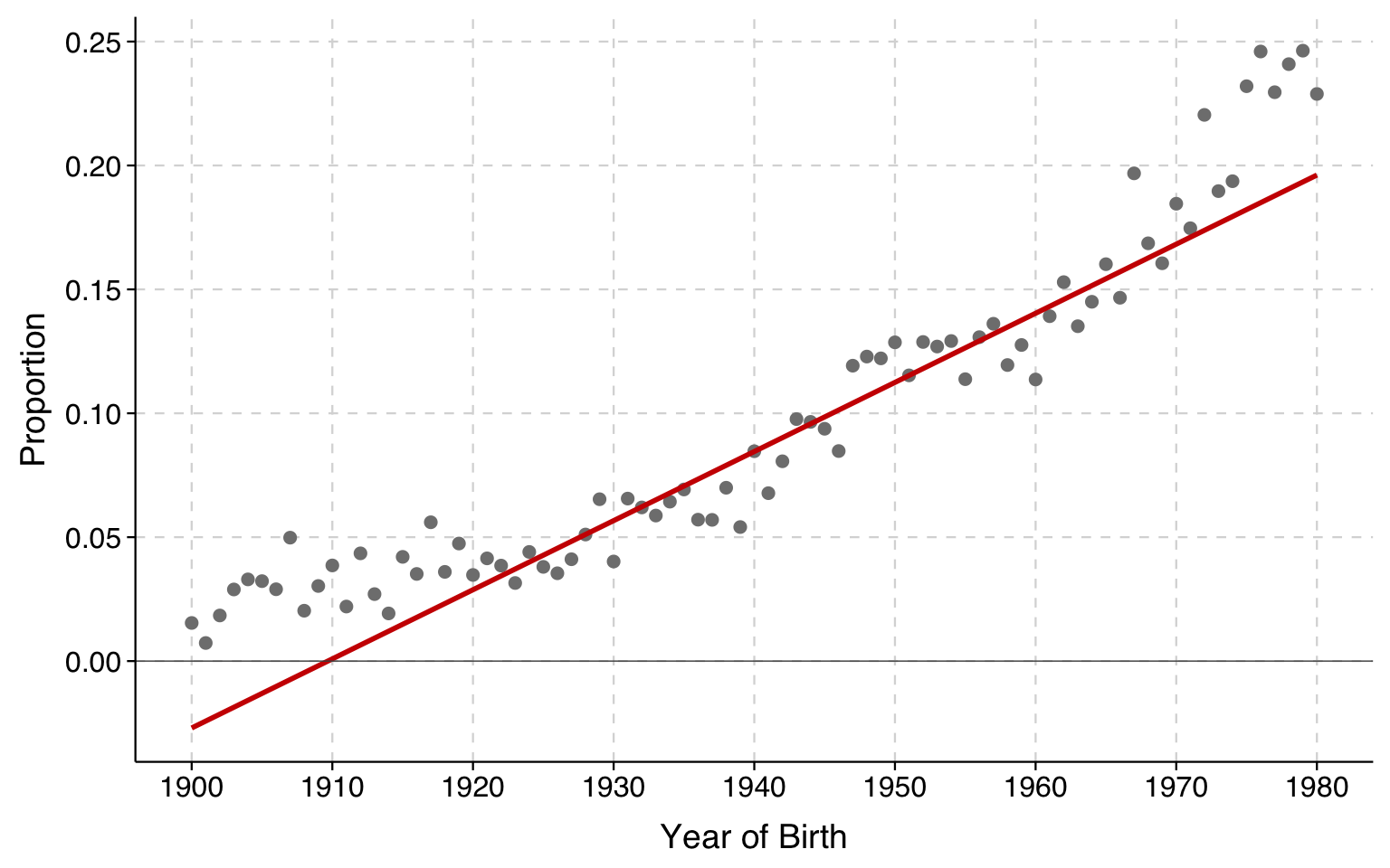
As another example, the graph below shows the proportion of religious nones by year of birth (1900–1980). The gray dots are the observed proportion for each year; the red line is the fitted LPM.
The model produces negative predicted probabilities for birth years prior to 1910, which is 3% of the observed cases in the data.
Unreasonable predictions are not uncommon in regressions with continuous outcomes, especially when one makes predictions using values of the explanatory variables that are outside the observed range. But impossible predictions are a different matter from merely unreasonable predictions. Worse, in practice, the linear probability model produces nonsense predicted values for plausible–or even observed–combinations of explanatory variables often enough to be distressing.
Advanced aside: The possibility of negative predicted probabilities introduces a technical complication, which is that sometimes people describe the linear probability model as being a generalized linear model with an identity link and binomial distribution. The usual way one would fit that model is using maximum likelihood. However, a negative predicted probability in that event would mean a negative likelihood, in which case the log-likelihood is undefined. In practice, this means that if one uses this technique to fit a linear probability model that would have negative predicted probabilities, the estimation procedure will either fail abruptly or run interminably without ever converging.
Problem #2: The LPM may be substantively unrealistic
Since the model is linear, a unit increase in \(x_{k}\) results in a constant change of \(\beta _{k}\) in the probability of an event, holding all other variables constant.
Imagine the amount of money a company would have to spend advertising a product in order to increase its market share by one percentage point. It seems reasonable to suppose that this would depend on how much market share the company already has. Specifically, we might imagine that it would cost less to move from 50% to 51% than from 1% to 2% (getting the product off the ground) or from 98% to 99% (converting the last few stragglers).
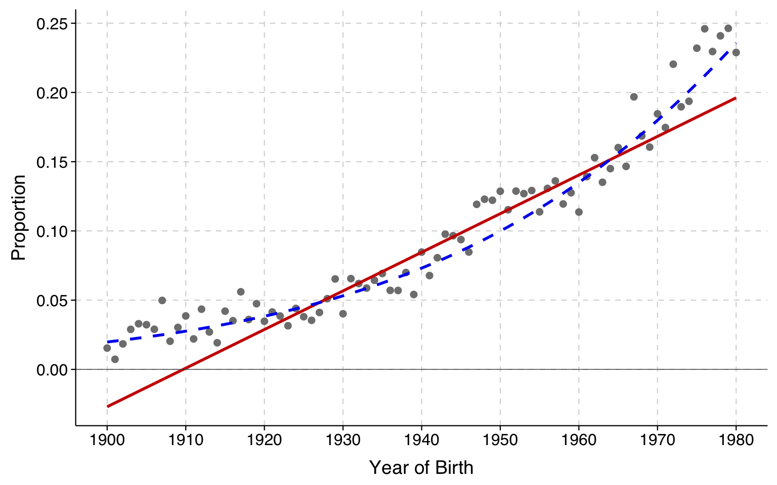
We can also think about this in terms of trends in a binary outcome. In our General Social Survey example, we are considering religious nones, something that used to be quite rare and is now far more common. For a trend like this, it seems implausible that it would take the same amount of time for a secular increase from 2% to 4% as an increase from 20% to 22%. Instead, in percentage point terms, we might expect trends to move more slowly when they are close to 0 and 1, and happen more rapidly as the trend approaches .5.
Indeed, let’s look again at the data on religious nones. If we draw a line in which the slope increases as we move away from 0, we fit the underlying proportions (gray dots) obviously better:
The blue dashed line is the fitted line from the logit model, which we will be introducing shortly.
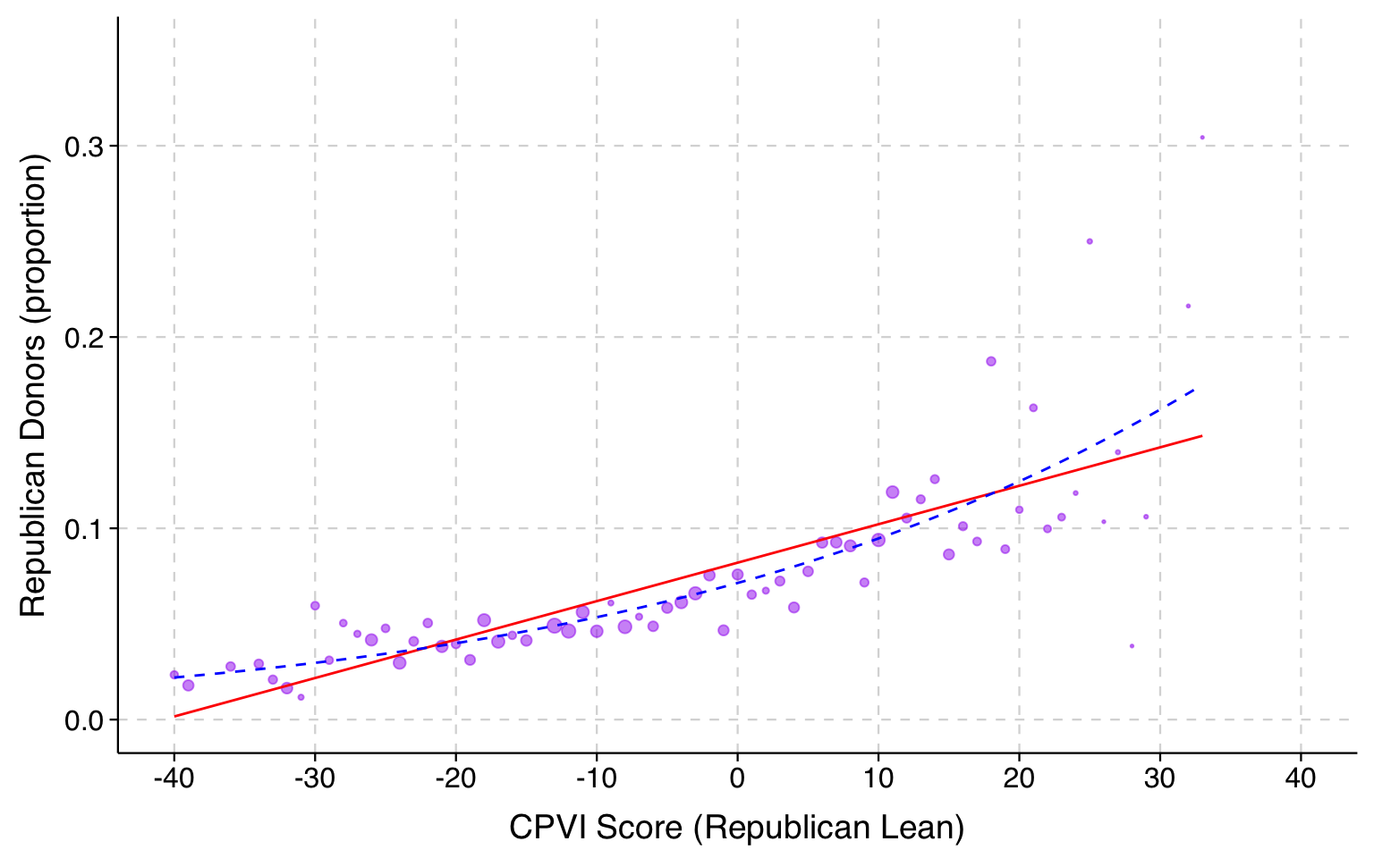
Second example: Political contributions data
The plot below uses the political contributions data from before.
In this case, we can see that the linear probability model (the red line) underpredicts the probabilities for the cases with the lowest values of the explanatory variable, and consistently underpredicts the probabilities in the middle.
When are the drawbacks of the LPM most apparent?
There are two ways of answering this. One is with respect to the data and explanatory variables one is working with, and one is with respect to what one hopes of learning from the analysis. In terms of the data and explanatory variables:
The model includes continuous variables (as opposed to only including categorical variables).
The explanatory variables have large effects on the probability of the outcome.
The data includes cases in which the predicted probabilities are under .2 or above .8—especially if they include cases under .1 or above .9.
On the other hand, if you have data in which the predicted probabilities are all intermediate values, especially all between .3 and .7 for the observed values in your data, the logit and probit models we will be considering are also very close to linear in the probabilities, and the substantive predictions from these models will look very similar to those of the linear probability model.
Meanwhile, in terms of the questions that one is asking, the drawbacks of the linear probability model are most apparent when one wants to predict or characterize the probability of the outcome at different values of the explanatory variables.
However, if all we cared about was the average change in probability between years—not the predicted probability at any particular point, or whether the rate of change is itself increasing—the drawbacks of the LPM are less apparent.