Predicted Change for a Continuous Explanatory Variable
In the logit model, the change in the predicted probability associated with a change in an explanatory variable depends on that variable’s baseline value.
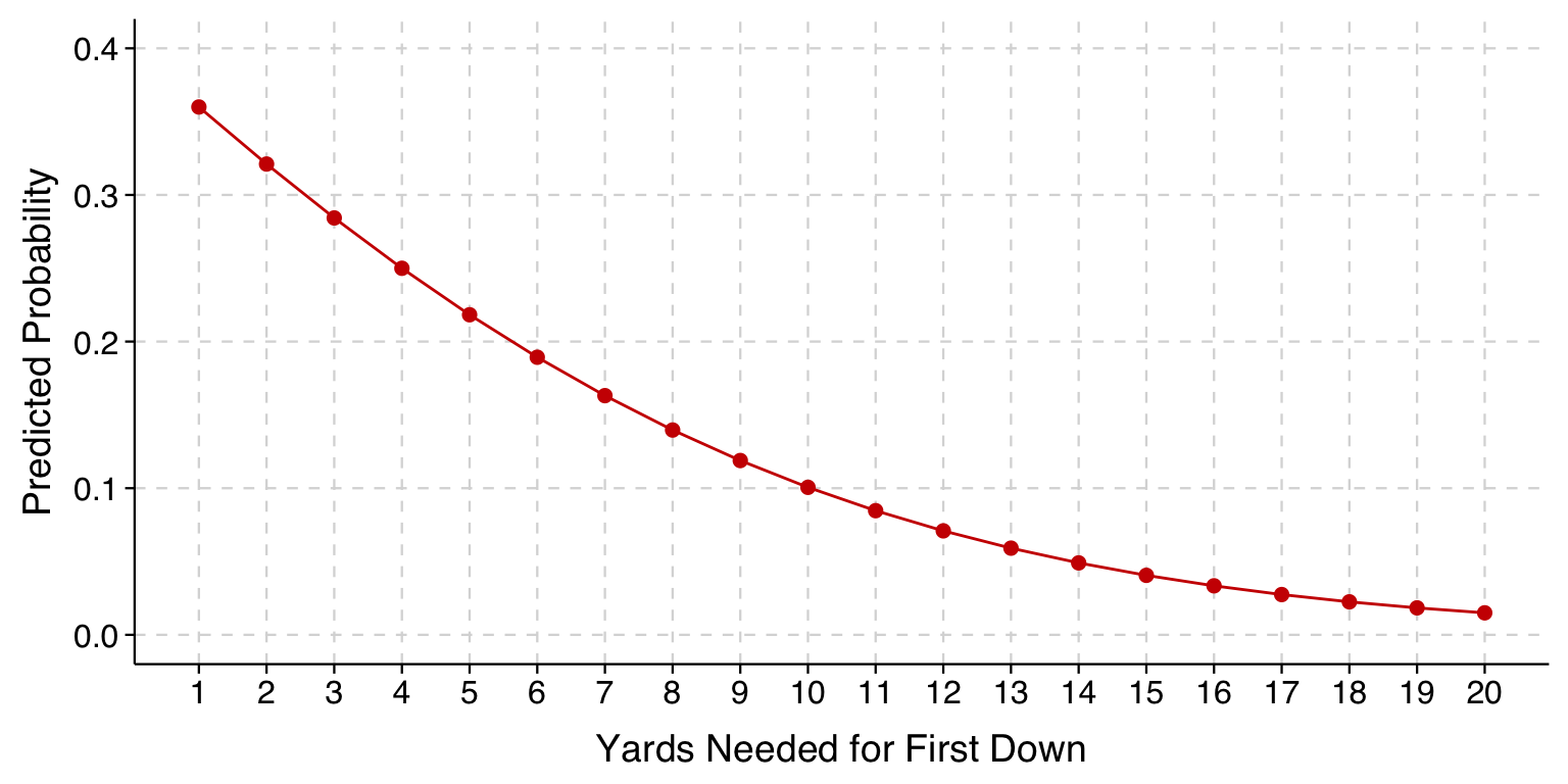
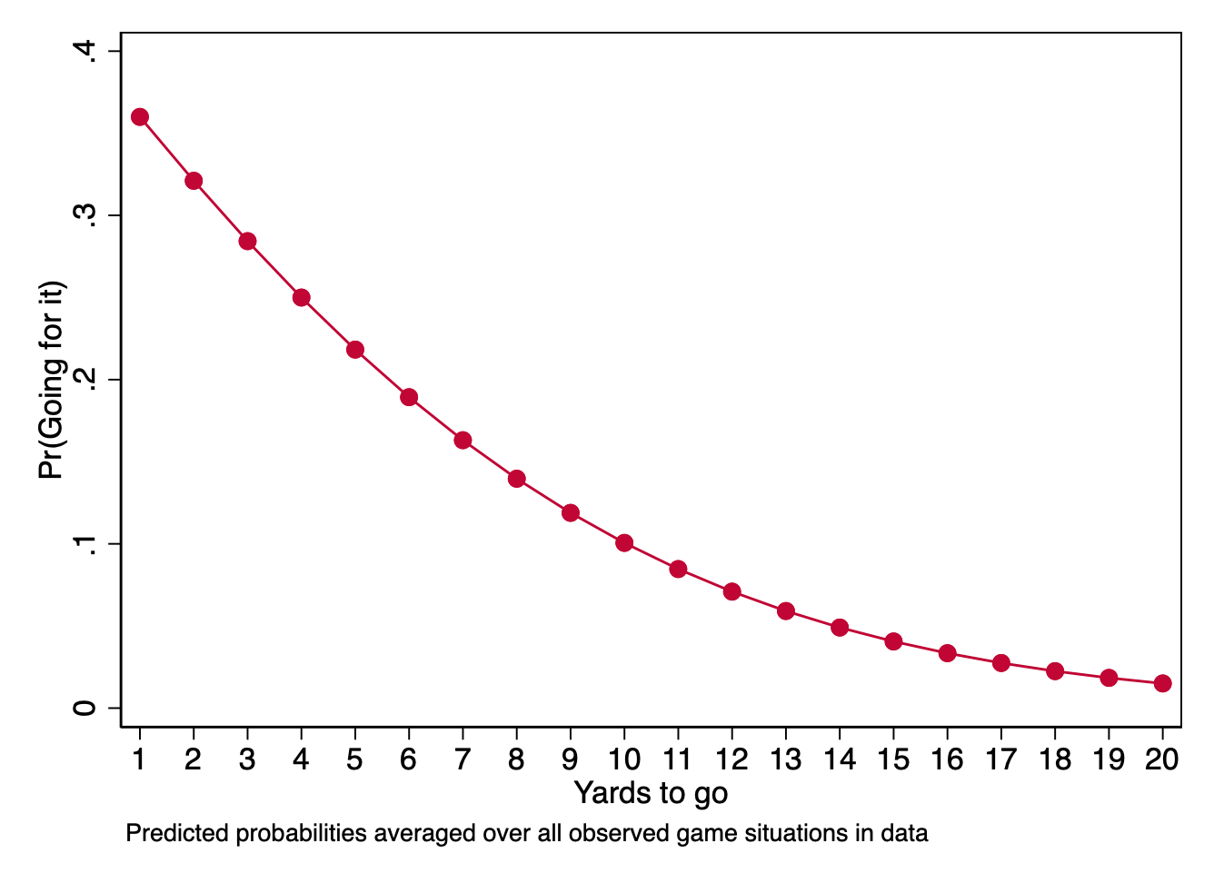
In the case of the earlier example of fourth-down decisions in football, we can see from the profile plot (reproduced below) that the difference that each additional yard needed makes in the probability of going for it shrinks as the distance increases. That is, the difference in predicted probabilities for a one-yard increase from 4th-and-1 to 4th-and-2 is larger than the difference for a one-yard increase from 4th-and-9 to 4th-and-10.
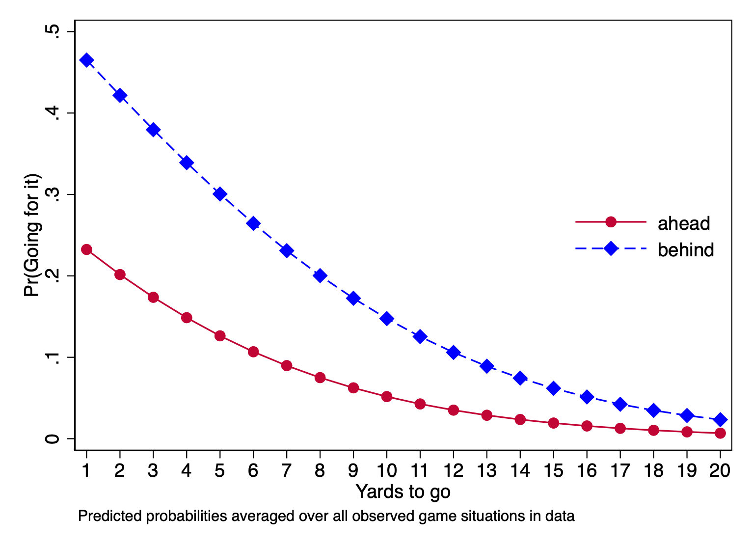
Moreover, the change in the predicted probability depends not just on the baseline value of our explanatory variable, but also on the values of the other explanatory variables. The profile below shows how the relationship between yards-to-go and the probability of going for it on fourth down also depends on whether the team is ahead or behind.
toplot <-avg_predictions(model,variables =c(list("yds_needed"=seq(1, 20, 1)), list("score_is"=c("ahead", "behind"))) )ggplot(toplot, aes(x = yds_needed, y = estimate, color = score_is, fill = score_is, linetype = score_is)) +geom_line() +geom_point(size =2, shape =21, stroke =1) +scale_color_manual(values =c("red3", "blue3"), name =NULL) +scale_fill_manual(values =c("red3", "blue3"), name =NULL) +scale_linetype_manual(values =c("solid", "dashed"), name =NULL) +scale_y_continuous(limits =c(0, 0.6)) +scale_x_continuous(limits =c(1, 20), breaks =seq(1, 20, 1),minor_breaks =NULL) +labs(x ="Yards Needed for First Down",y ="Predicted Probability" ) +theme_tula() +theme(legend.position =c(0.95, 0.95),legend.justification =c(1, 1),legend.background =element_rect(fill ="white", color ="gray80",linewidth =0.5, linetype ="solid"),legend.margin =margin(6, 6, 6, 6),panel.grid.minor =element_blank() )
If we look now at the difference in predicted probabilities between 4th-and-1 and 4th-and-2, we can see that it is bigger when the team is behind than it is when the team is ahead.
Marginal change
For continuous explanatory variables, changes in predicted probability are often presented in terms of marginal changes (or “marginal effects”). If you have had some calculus, the marginal change is the derivative evaluated at specific values of explanatory variable(s) \(\mathbf{x}\).
If you haven’t had calculus, look at the first profile plot above. The slope of the curve representing the predicted probabilities decreases as distance increases. At any point along that curve, we can evaluate the slope of the curve at that specific point. (Imagine magnifying the curve at any specific spot–if you magnify enough, any curve examined at a single, specific point will look like a straight line, and we are asking what the slope of that straight line is.)
You will be reasonably close if you think of the marginal effect as the change in \(y\) for a unit change in \(x\) evaluated at some particular point.
Stata: Average change for one-unit change in explanatory variable. I have co-authored a command for Stata that computes the average change for a one-unit change instead of the marginal change. The command is called \(\mathtt{mchange}\) and is available as part of the \(\mathtt{spost13\_ado}\) package available online using the \(\mathtt{findit}\) command in Stata.
Again, I think for practical purposes the marginal change approximates this closely enough except when the scale of the explanatory variable is very small (i.e., when your explanatory variable is a proportion or something else that only varies from 0 to 1).
Marginal change in logit
The marginal change for an explanatory variable is calculated given specific values of all the explanatory variables.
The formula for the marginal change in the logit model is simple. For explanatory variable \(x\), the change in \(Pr(y=1)\) for a marginal increase in \(x\) is a function of two things:
the logit coefficient of \(x\) (\(\beta_x\))
the predicted probability of y=1 given specific value(s) of the explanatory variable(s) (that is, \(\Pr(y=1|\mathbf{x})\)).
Specifically, the formula is: \[
\mathrm{Marginal\ change\ for\ }x = \beta_x\left[\Pr(y=1|\mathbf{x})\right]\left[1-\Pr(y=1|\mathbf{x})\right]
\]
We can see from this formula why the marginal change depends on the values of all the explanatory variables: it depends on \(\Pr(y=1|\mathbf{x})\), and \(\Pr(y=1|\mathbf{x})\) depends on the values of all the explanatory variables.
Also, notice that, for a given value of \(\mathbf{x}\) – that is, a given value of \(\Pr(y=1|\mathbf{x})\) – the marginal changes for all the explanatory variables will differ from one another exactly in proportion to their coefficients.
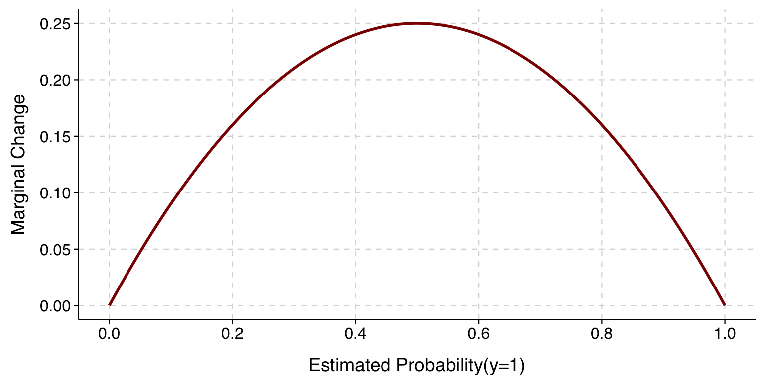
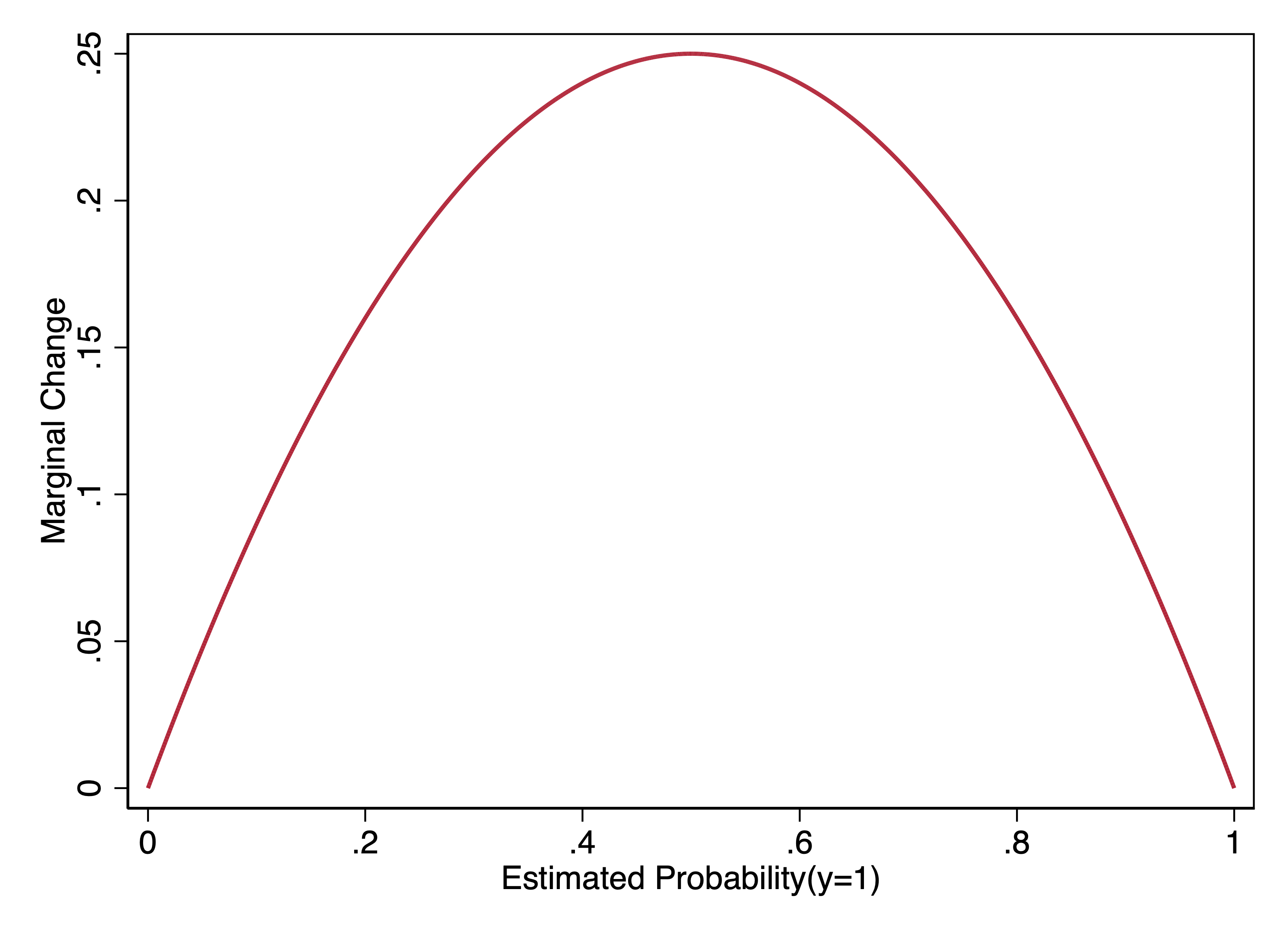
Using this formula, we can plot, over the whole range of possible predicted probabilities, the marginal change when \(\beta=1\).
We can see here that the marginal change is biggest when \(\Pr(y=1)\) is .5, and it is smallest as \(\Pr(y=1)\) approaches either 0 or 1.
Moreover, when \(\Pr(y=1)\) is .5, not only is the marginal effect the biggest, but it is equal to \(\beta_x\) times .25. This means that if you divide a logit coefficient by 4, you get the maximum (in magnitude) marginal effect. This is sometimes called the “divide by 4 rule”.
Two other observations from the curve above:
The marginal change when \(\Pr(y=1) = p\) has the same magnitude as when \(\Pr(y=1) = 1-p\).
The curve above gets steeper as the predicted probability approaches 0 or 1. As a result, the marginal effects when \(\Pr(y=1)\) is between .4 and .6 vary much less than, say, when the predicted probability varies between 0 and .2.
Average marginal change
The marginal change for an explanatory variable could be different for every observation in our dataset. For our college football example of going for it on fourth down, we can calculate the marginal change for the \(\mathtt{yds\_needed}\) variable for every observation and make a histogram to show this variation. We can look at it alongside a histogram of the predicted probabilities in these data.
Expand to show code that draws histograms
compute_me <-predictions(model, type ="response") %>%rename(pr_1 = estimate) %>%mutate(pr_0 =1- pr_1) %>%mutate(marg_eff =coef(model)["yds_needed"] * pr_1 * pr_0)p1 <-ggplot(compute_me, aes(x = marg_eff)) +geom_histogram(fill ="deepskyblue", color ="black", bins =50) +labs(x ="Marginal change for yds_needed",y ="Frequency" ) +theme_tula()p2 <-ggplot(compute_me, aes(x = pr_1)) +geom_histogram(fill ="gold", color ="black", bins =50) +labs(x ="Predicted probability of going for it",y ="Frequency" ) +theme_tula()grid.arrange(p1, p2, ncol =2)
Things to notice about these graphs:
Looking at the left graph, you’ll notice that the marginal changes are all negative. This is because the coefficient of \(\mathtt{yds\_needed}\) is negative. In a binary outcome model, the marginal change for a variable is always the same sign as the coefficient of that variable.
The distribution of marginal changes in the left graph has two peaks (on each end), whereas the distribution of predicted probabilities in the right graph has only one.
The peak on the right side of the marginal change plot reflects the large number of cases with predicted probabilities near 0. Because the predicted probability is near zero, the marginal change is near zero as well.
The peak on the left side of the marginal change plot, on the other hand, reflects cases that have predicted probabilities around .5. Because a relatively wide interval of predicted probabilities around .5 has similar marginal changes, these observations add up and create a peak even though the number of cases at any specific predicted probability in that interval is relatively few.
The average marginal change (also called the average marginal effect and often abbreviated as AME) is the mean of the marginal changes for each observation.
Here we will calculate the average marginal change ourselves by computing the marginal change for each observation and then calculating the mean.
. predict pr_1 if e(sample)
(option pr assumed; Pr(goforit))
(6,399 missing values generated)

. gen me = _b[yds_needed] * pr_1 * (1-pr_1)
(6,399 missing values generated)

. sum me // average marginal change

    Variable |        Obs        Mean    Std. dev.       Min        Max
-------------+---------------------------------------------------------
          me |     80,887    -.024438    .0176084  -.0534086   -.000043
In practice, we would instead have Stata compute the average marginal change using \(\texttt{margins, dydx()}\), as follows:
. margins, dydx(yds_needed)

Average marginal effects                                Number of obs = 80,887
Model VCE: OIM

Expression: Pr(goforit), predict()
dy/dx wrt:  yds_needed

------------------------------------------------------------------------------
             |            Delta-method
             |      dy/dx   std. err.      z    P>|z|     [95% conf. interval]
-------------+----------------------------------------------------------------
  yds_needed |   -.024438   .0003041   -80.36   0.000     -.025034   -.0238419
------------------------------------------------------------------------------
We can interpret this result as:
Averaging over all observed game situations, the decrease in the probability of going for it on fourth down for a marginal increase in yards needed is -.024, net of field position, quarter, and which team is leading.
If we want to fudge to make it a bit more accessible:
Averaging over all observed game situations, an additional yard is associated with about a .024 decrease in the probability of going for it on fourth down, net of field position, quarter, and which team is leading.
Aside: Why do I say “marginal change” when one more often sees “marginal effect”? In social science, it is very common that people will use “effect” when describing coefficients while still being adamant that they are not actually saying anything about causality. I do this, too, but have been endeavoring to wean myself off of it.
Stata: What does the \(\texttt{dydx()}\) option for \(\texttt{margins}\) do? The \(\texttt{dydx()}\) option can be confusing because it effectively does two different things:
For a continuous variable – and Stata will assume the variable is continuous unless you specify \(\texttt{i.}varname\) when fitting the model – \(\texttt{margins, dydx(}varname\texttt{)}\) will provide the marginal change for \(varname\).
For a factor variable, Stata will instead provide the change in the outcome associated with a change in the factor variable from its reference category to the specified category (so, for a binary explanatory variable, the change in \(\Pr(y=1)\) as \(x\) changes from 0 to 1).
Again, whether a variable is treated as continuous or as a factor variable depends on whether you specified \(\texttt{i.}\) when fitting the model. You do not specify \(\texttt{i.}\) again when using \(\texttt{margins}\); it “remembers” based on what you specified when you fit the model.
The \(\texttt{dydx}\) is a calculus reference, referring to the idea of the derivative as the rate of change in \(y\) evaluated at a particular value for x.
Average marginal change as approximation of the average change for a unit increase
The marginal change will be very close to the change associated with a unit increase in \(x\) when the scale of a variable is large enough that a unit increase is a relatively small change in the variable.
The marginal change will be a worse approximation of the change associated with a unit increase when the scale is small, so that a unit increase is a big change in the explanatory variable. Worst of all is when the scale is so small that a unit change in an explanatory variable is bigger than its entire range (like, for example, if your explanatory variable is a proportion).
In R, you can obtain the average change for a unit increase instead of the average marginal change by adding eps = 1 as an argument to avg_comparisons.
The average change is -.0244, or the same at this level of precision as the average marginal effect. So when I described the above interpretation in terms of the change in probability associated with an additional yard as being a “fudge,” it turns out that in this case it was not a fudge at all.
Average marginal change and the coefficient of the linear probability model
In the linear probability model, the \(\beta\) coefficient is the marginal change in the probability, and, unless we are using some kind of nonlinear specification of the explanatory variables, the marginal change for an explanatory variable is the same across all values of the explanatory variables.
Since the marginal change in the linear probability model is estimated to be the same across all observations, we can refer to the coefficient as the linear probability model’s estimate of the average marginal change.
The average marginal change as estimated by the linear probability model is \(-.017\), as opposed to \(-.024\) from the logit model. This is about a 30% difference, which I would not consider substantively trivial, especially given that the large number of cases means our standard errors are very small. But, many times, the estimates will be closer than this, especially for models where the predicted probabilities are all in the middle of the distribution and so the marginal effects from logit will not vary that much anyway.
Earlier in the class we noted that when predicted probabilities are all in the middle of the distribution (say, .3 to .7), a linear change in the probabilities looks a lot like the predictions of the logit model. In those cases, the coefficient from the linear probability model will also be close to the average marginal effect from the logit model, strengthening the argument that just using the linear probability model in that case will probably not lead to any substantive mischaracterization of results.
Marginal change differences by groups
Above we showed a graph in which the relationship between yds_needed and going for it was stronger when a team was behind versus ahead.
In R, we can compute average marginal change of a continuous variable by different groups by adding a by argument to avg_comparisons.