Probit regression and the latent variable approach to binary outcomes
In the latent variable approach to binary outcomes, the binary outcome is treated as observed dichotomous manifestation of an underlying and unobserved continuous variable.
For example, the General Social Survey asks respondents “Do you favor or oppose the death penalty for persons convicted of murder?” Respondents are only given two ways of answering this question – favor or oppose. Instead, the question could have the answer categories of “strongly favor”, “slightly favor”, “slightly oppose,” or “strongly oppose.” Or more categories for more gradations.
In the latent variable approach, we posit that respondents have, in reality, an attitude of (say) favorability toward capital punishment that can be placed on a continuum. But we do not observe this favorability directly. All we observe is the binary answer of favor or oppose.
Then, we imagine that the binary variable we observe maps onto the underlying continuous variable by way of a threshold. In our example, if respondent’s underlying favorability is above the threshold, they say “favor.” If it is below the threshold, they say “oppose.”
The probit model
To put this in more formal terms, \(y\) is the binary variable that we observe (1=“favor”, 0=“oppose”) We use \(y^*\) (“y star”) to represent our latent variable (respondent favorability toward capital punishment). We use \(\tau\) (tau) to represent the threshold.
This is just like the familiar linear regression model–including an error term!–only except for our outcome being observed it is now latent.
As in linear regression, we will assume the error term is normally distributed with constant variance and a mean of 0.
A big difference with linear regression is that in linear regression the standard deviation of the error term is estimated from our observed data–it is the RMSE. In the probit model, because our outcome is unobserved, we have to assume a value for this standard deviation. We use 1 because this means that the errors are distributed as the standard normal and that is simplest.
Aside: The formal way of writing that we assume that the errors are normally distributed with a mean of 0 and standard deviation of 1 is:
\(\varepsilon \sim N(0, 1)\)
where \(N\) is understood in this context to indicate the normal distribution and \(\sim\) means “is distributed as”
We will also keep things simplest by assuming that \(\tau\) is 0. This is completely arbitrary and will have no substantive implications for our results. So,
\(y=1\) if \(y^*> 0\)
\(y=0\) if \(y^*< 0\)
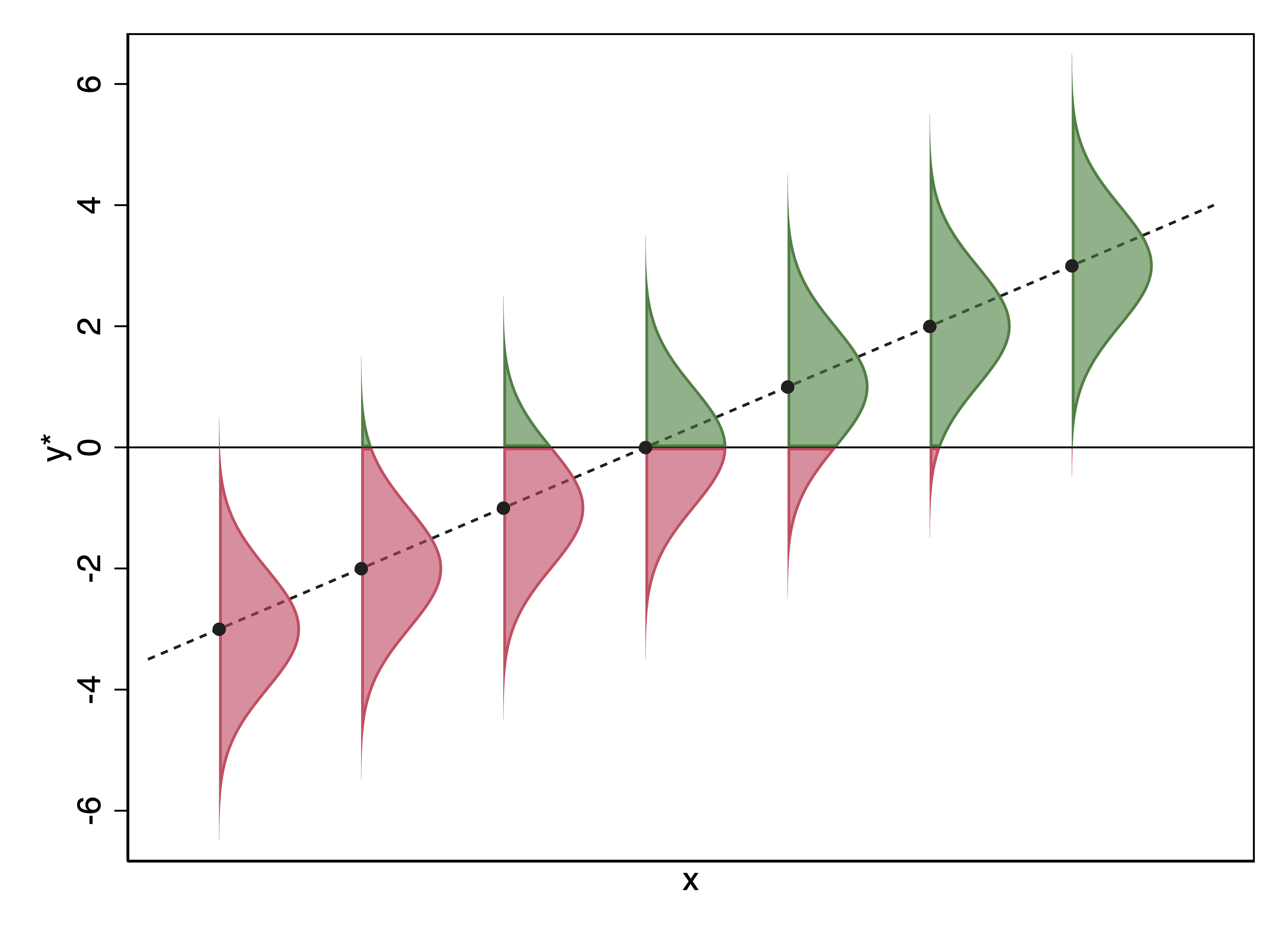
Understanding this graph will drive home what is going on conceptually:
The dotted line is a hypothetical regression line, showing how \(\mathbf{x}\mathbf{\beta}\) changes with respect to an explanatory \(x\). (\(\beta_x\) must be positive given that \(x\beta\) is sloping upward.)
The black dots represent \(\mathbf{x}\mathbf{\beta}\) at particular values of \(\mathbf{x}\). For each value of \(\mathbf{x}\mathbf{\beta}\), there is an distribution of \(\varepsilon\) that is a standard normal distribution.
We observe \(y = 1\) if \(y^* > 0\), and \(y = 0\) if \(y^* < 0\). The probability of \(y = 1\) given \(\mathbf{x}\mathbf{\beta}\) is the portion of the corresponding normal curve that is above 0. This is depicted in green in the graph, while the probability that \(y = 0\) (\(y^* < 0\)) is depicted in red.
Our regression line is upward sloping, meaning that as \(\mathbf{x}\mathbf{\beta}\) increases, more of the normal curve falls over the threshold. This means that the predicted probability that \(y = 1\) is increasing.
Probability of \(y = 1\) in the probit model
For a given observation, \(y_i=1\) if \(y^* > 0\), which means that if \(\mathbf{x}\mathbf{\beta} + \varepsilon > 0\).
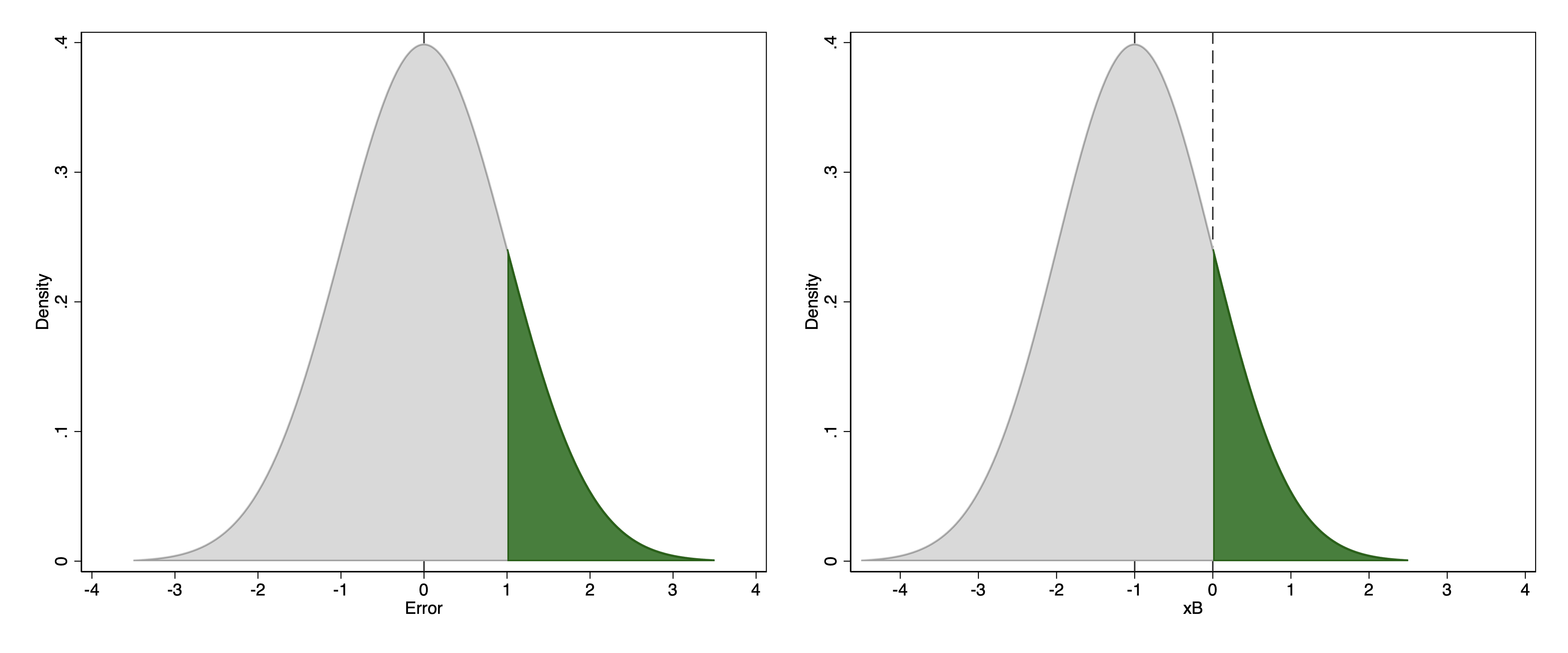
Consider, for example, an observation in which \(\mathbf{x}\mathbf{\beta}\) is \(-1\).
This observation will have a positive outcome (\(y=1\)) if \(-1 + \varepsilon > 0\).
The probability of a positive outcome, therefore, is the probability that \(\varepsilon > 1\).
Because \(\varepsilon\) follows a standard normal distribution, the probability that \(y = 1\) given that \(\mathbf{x}\mathbf{\beta} = -1\) if the probability of observing a value greater than 1 in a random draw from a standard normal distribution.
The left-hand graph above depicts the probability that \(\varepsilon > 1\) given the standard normal distribution. The right-hand graph shows this in terms of drawing the standard normal distribution centered on \(\mathbf{x}\mathbf{\beta}=-1\) and then highlighting the part of the distribution that is greater than the threshold value of 0.
We can obtain this using the cumulative distribution function for the normal distribution that we talked about before. In Stata, the area to the left of \(z\) in the standard normal can be obtained using the function \(\mathtt{normal(}z\mathtt{)}\). In our case, we want the area to the right of z, so we take \(1 - \mathtt{normal(}z\mathtt{)}\) instead.
::::: {.panel-tabset group="software"}

# Stata

. display 1 - normal(1)
.15865525

# R


::: {.cell}

```{.r .cell-code}
# In R, pnorm() is the cumulative distribution function for the normal distribution
# The area to the right of z=1 is 1 - pnorm(1)
1 - pnorm(1)
```

::: {.cell-output .cell-output-stdout}

```
[1] 0.1586553
```


:::
:::


:::::
Because the standard normal distribution is symmetric around 0, \(1 - \mathtt{normal(}z\mathtt{)}\) is the same as \(\mathtt{normal(}-z\mathtt{)}\), so we could have obtained the same answer by typing:
::::: {.panel-tabset group="software"}

# Stata

. display normal(-1)
.15865525

# R


::: {.cell}

```{.r .cell-code}
# Using the symmetry of the standard normal distribution
pnorm(-1)
```

::: {.cell-output .cell-output-stdout}

```
[1] 0.1586553
```


:::
:::


:::::
More generally, if we use \(\mathtt{cdf\_normal}\) to refer to the cumulative distribution function of the normal distribution:
That last equation means that the probability of a positive outcome given is just the cumulative distribution function for the standard normal:
Key point: The probability that \(y=1\) in the probit model is \(\mathtt{cdf\_normal}(\mathbf{x}\mathbf{\beta})\).
Simple illustration
In this example, we will look at data from NCAA Division I women’s lacrosse matches over five seasons (2014-2018). Our outcome is whether or not the team won the game. Our explanatory variable is how many goals the team scored.
── Attaching core tidyverse packages ──────────────────────── tidyverse 2.0.0 ──
✔ dplyr     1.2.0     ✔ readr     2.2.0
✔ forcats   1.0.1     ✔ stringr   1.6.0
✔ ggplot2   4.0.2     ✔ tibble    3.3.1
✔ lubridate 1.9.5     ✔ tidyr     1.3.2
✔ purrr     1.2.1
── Conflicts ────────────────────────────────────────── tidyverse_conflicts() ──
✖ dplyr::filter() masks stats::filter()
✖ dplyr::lag()    masks stats::lag()
ℹ Use the conflicted package (<http://conflicted.r-lib.org/>) to force all conflicts to become errors
library(haven)# Load datadf <-read_dta("../dta/wlax-scores.dta") %>%filter(!is.na(home_score)) %>%filter(!is.na(away_score))# Create binary outcome: home team winsdf <- df %>%mutate(home_win =ifelse(home_score > away_score, 1, 0))# Fit probit modelmodel_probit <-glm(home_win ~ home_score,data = df,family =binomial(link ="probit"))summary(model_probit)
Call:
glm(formula = home_win ~ home_score, family = binomial(link = "probit"),
    data = df)

Coefficients:
             Estimate Std. Error z value Pr(>|z|)
(Intercept) -3.315744   0.080813  -41.03   <2e-16 ***
home_score   0.306557   0.007099   43.18   <2e-16 ***
---
Signif. codes:  0 '***' 0.001 '**' 0.01 '*' 0.05 '.' 0.1 ' ' 1

(Dispersion parameter for binomial family taken to be 1)

    Null deviance: 8063.4  on 5891  degrees of freedom
Residual deviance: 4424.2  on 5890  degrees of freedom
AIC: 4428.2

Number of Fisher Scoring iterations: 6
logLik(model_probit)
'log Lik.' -2212.114 (df=2)
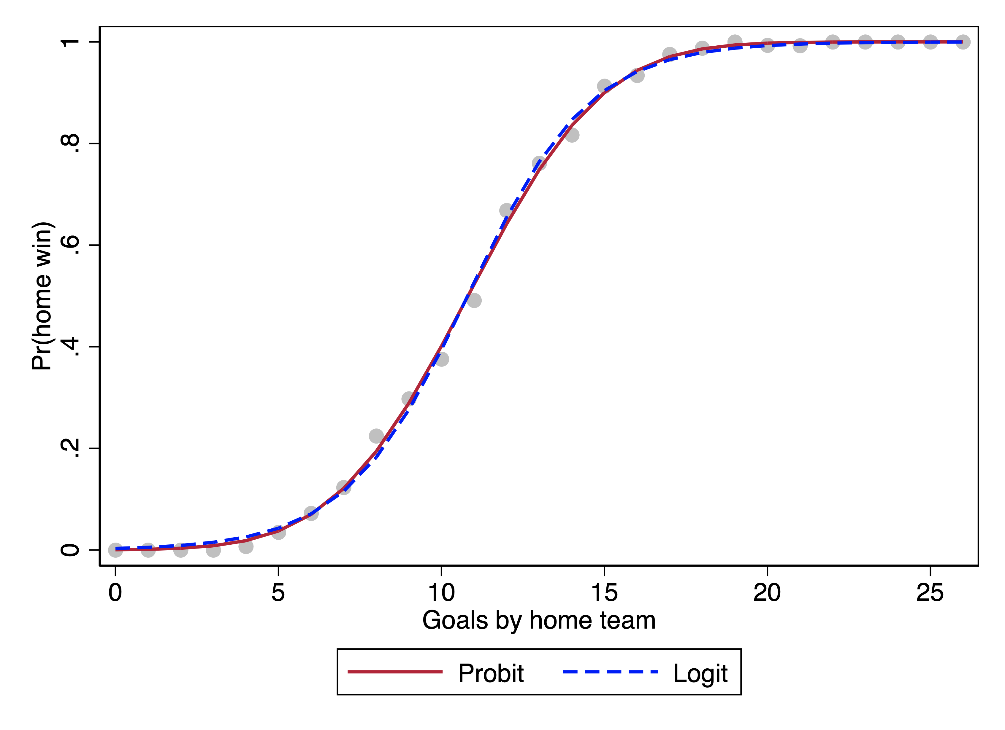
If the home team scores ten goals, \(\mathbf{x}\mathbf{\beta}\) would be \(-3.315 + 3.065 = -.250\). This corresponds to a predicted probability of .401. In other words, when the home team scores 10 goals, we predict they have a 40.1% chance of winning.
The graph below shows the predicted probability of victory over the entire range of goals, and we can see that it corresponds closely to the observed proportion of wins (the gray circles) throughout.
Interpreting probit results
Probit coefficients, on their own, do not have any especially accessible interpretation. In the same way that untransformed logit coefficients can be interpreted as changes in log odds, probit coefficients can be interpreted as “probits.”
Again, and emphatically, odds ratios are only for logit models. Exponentiating probit coefficients is not something that results in a meaningful quantity. There is a technique for transforming a probit coefficient to a more meaningful quantity that we will talk about later.
The various techniques that we showed for interpretations using predicted probabilities for the logit model also can be used with probit models.
Binary logit as a latent variable model
We used the latent variable approach to introduce the probit model for binary outcomes. Probit is an appealing way of presenting the latent variable approach because the probit model is based on the normal distribution, and we are used to thinking about normally distributed errors from linear regression.
However, we can also develop the binary logit model using the latent variable approach. To do this, we follow the same logic as the model above, but change two assumptions about the error term:
We do not assume the normal distribution for the error term, but the logistic distribution. The logistic distribution is similar in shape to the normal distribution, but it is not identical.
We do not assume that the standard deviation of the errors is 1, but we assume the standard deviation is \(\frac{\pi}{\sqrt{3}}\).
Neither of these assumptions is a straightforward as the counterpart in probit, but these changes are necessary to make the model equivalent to the logit model, in which \(\mathbf{x}\mathbf{\beta}\) is the logged odds of a positive outcome.
The fact that when we write the logit model as a latent variable model we assume a larger standard deviation for the errors account for one difference between the results of logit and probit models. When fitting the same outcome with the same explanatory variables, logit coefficients will be bigger in magnitude than probit coefficients by a factor of 1.5 to 2. You can think of this as the logit model having a smaller scale than the probit model, the way that coefficients for weight will all be bigger if our outcome is weight measured in pounds rather than weight measured in kilograms, even though substantively nothing changes.
In our model of women’s lacrosse outcomes, the slope in the probit model was .306. In the logit model:
# Fit logit model on the same datamodel_logit <-glm(home_win ~ home_score,data = df,family =binomial(link ="logit"))summary(model_logit)
Call:
glm(formula = home_win ~ home_score, family = binomial(link = "logit"),
    data = df)

Coefficients:
            Estimate Std. Error z value Pr(>|z|)
(Intercept)  -5.7836     0.1553  -37.23   <2e-16 ***
home_score    0.5353     0.0138   38.79   <2e-16 ***
---
Signif. codes:  0 '***' 0.001 '**' 0.01 '*' 0.05 '.' 0.1 ' ' 1

(Dispersion parameter for binomial family taken to be 1)

    Null deviance: 8063.4  on 5891  degrees of freedom
Residual deviance: 4432.9  on 5890  degrees of freedom
AIC: 4436.9

Number of Fisher Scoring iterations: 6
logLik(model_logit)
'log Lik.' -2216.437 (df=2)
Yet, despite the differences in the magnitude of coefficients, when we translate each to predicted probabilities, the predictions are very similar:
What this illustrates is that, substantively, logit and probit models for binary outcomes imply very similar predicted probabilities. Not exactly the same, but close. In my experience, if you run and logit model and a probit model and look at the correlation of predicted probabilities between the two, the result is \(r = .99\) or more.
For this reason, there is basically no reason with ordinary survey data to prefer logit or probit because one will give you more accurate estimates or reliably fit the data better. With a Big Data application, maybe?