Expand for code that loads packages
library(tidyverse)
library(haven)
library(tulaverse)
library(lmtest)
library(sandwich)
library(car) # needed for linearHypothesis() function used later
library(restriktor) # used for constrained estimationThe most frequently invoked use of hypothesis testing in regression models is the test of whether a coefficient is zero. This is the test represented by the p-value in standard regression output.
But there are other tests, including whether a set of coefficients are simultaneously equal to zero, whether a coefficient is equal to some value other than zero, and whether the coefficients for two different variables are equal to each other.
When we fit a model using maximum likelihood, the likelihood function provides the basis for statistical hypothesis testing. There are three key ways this is done: the likelihood-ratio test, the Wald test, and the score test.
We will focus only on the first two. The likelihood-ratio test is the more intuitive of the two, and we will introduce it first. Also, in cases where both tests are appropriate, advice tends toward preferring the likelihood-ratio test. However, there are important cases where Wald tests remain appropriate when likelihood-ratio tests are not, so one cannot simply always rely on the likelihood-ratio test.
Here are estimates from our analysis of data on the survival of passengers on the Titanic:
library(tidyverse)
library(haven)
library(tulaverse)
library(lmtest)
library(sandwich)
library(car) # needed for linearHypothesis() function used later
library(restriktor) # used for constrained estimationdf <- read_dta("../dta/titanic_passengers.dta") %>%
mutate(female = as_factor(female)) %>%
mutate(child = as_factor(child)) %>%
mutate(pclass = relevel(as_factor(pclass), ref = "3rd"))model_unconstrained <- glm(survived ~ female + child + pclass,
data = df,
family = binomial(link = "logit"))
tula(model_unconstrained)Family: binomial / Link: logit
AIC = 1244.587 Number of obs = 1309
BIC = 1270.472 McFadden R-sq = 0.2909
Log likelihood = -617.293 Nagelkerke R-sq = 0.4362
─────────────────────────────────────────────────────────────────────────────
survived │ Coef Std. Err. z P>|z| [95% Conf Interval]
─────────────────────────────────────────────────────────────────────────────
female │ 2.499 .1484 16.84 <.0001 2.208 2.79
child │ 1.085 .2292 4.735 <.0001 .636 1.535
pclass │
1st │ 1.862 .1761 10.57 <.0001 1.517 2.207
2nd │ .8977 .1802 4.981 <.0001 .5445 1.251
(Intercept) │ -2.295 .1353 -16.96 <.0001 -2.56 -2.029
─────────────────────────────────────────────────────────────────────────────. logit survived i.female i.child ib3.pclass, nolog
Logistic regression Number of obs = 1,309
LR chi2(4) = 506.44
Prob > chi2 = 0.0000
Log likelihood = -617.29343 Pseudo R2 = 0.2909
------------------------------------------------------------------------------
survived | Coefficient Std. err. z P>|z| [95% conf. interval]
-------------+----------------------------------------------------------------
female |
female | 2.499297 .1483849 16.84 0.000 2.208467 2.790126
|
child |
child | 1.085262 .2292127 4.73 0.000 .636013 1.53451
|
pclass |
1st | 1.861954 .1760938 10.57 0.000 1.516816 2.207091
2nd | .8976734 .1802103 4.98 0.000 .5444676 1.250879
|
_cons | -2.294625 .1352986 -16.96 0.000 -2.559805 -2.029445
------------------------------------------------------------------------------
In these results, the estimate for \(\texttt{child}\) is 1.085. This is reported with a z-statistic of 4.73 and a p-value of .000 (meaning \(<.0005\)).
The p-value here evaluates the null hypothesis that the coefficient of \(\texttt{child}\) is 0, and its very low value indicates that it is very unlikely that we would observe a sample estimate as big as 1.085 by chance if the population parameter truly was 0. Consequently, we have evidence that the coefficient is greater than 0; that is, that children were indeed more likely to survive the sinking of the Titanic at a rate beyond what could be explained by pure chance.
What we are going to do here is show how we could get to the same conclusion using the likelihood. We will not end up with exactly the same result, but we will be close, and I will explain why later.
For now, take note of the log-likelihood of the model that we’ve fit: \(-617.29343\).
Testing a null hypothesis can be thought of as evaluating the estimates we observed vs. what we would have observed if we imposed some constraint(s) on our estimates.
In the case of the null hypothesis that \(\beta_\texttt{child} = 0\), our constrained model is one in which the coefficient of \(\texttt{child}\) is forced to be 0. We can obtain maximum likelihood estimates as before, but now under the constraint that the coefficient for child is 0.
This is easy enough to do:
model <- glm(survived ~ female + child + pclass,
             data = df, family = "binomial")
tula(model)
Family: binomial / Link: logit
AIC = 1244.587 Number of obs = 1309
BIC = 1270.472 McFadden R-sq = 0.2909
Log likelihood = -617.293 Nagelkerke R-sq = 0.4362
─────────────────────────────────────────────────────────────────────────────
survived │ Coef Std. Err. z P>|z| [95% Conf Interval]
─────────────────────────────────────────────────────────────────────────────
female │ 2.499 .1484 16.84 <.0001 2.208 2.79
child │ 1.085 .2292 4.735 <.0001 .636 1.535
pclass │
1st │ 1.862 .1761 10.57 <.0001 1.517 2.207
2nd │ .8977 .1802 4.981 <.0001 .5445 1.251
(Intercept) │ -2.295 .1353 -16.96 <.0001 -2.56 -2.029
─────────────────────────────────────────────────────────────────────────────constrained <- restriktor(model, constraints = "childchild == 0")
tula(constrained)Constrained / Family: binomial / Link: logit
Log likelihood = -628.611 Number of obs = 1309
McFadden R-sq = 0.2909
Num. constraints = 1
─────────────────────────────────────────────────────────────────────────────
survived │ Coef Std. Err. t P>|t| [95% Conf Interval]
─────────────────────────────────────────────────────────────────────────────
female │ 2.515 .1467 17.14 <.0001 2.227 2.803
child │ 0 0 0 1.0000 0 0
pclass │
1st │ 1.723 .1715 10.05 <.0001 1.387 2.06
2nd │ .8423 .1776 4.743 <.0001 .4939 1.191
(Intercept) │ -2.129 .1268 -16.79 <.0001 -2.378 -1.88
─────────────────────────────────────────────────────────────────────────────. constraint define 1 1.child = 0
. logit survived i.female i.child ib3.pclass, constraint(1) nolog
Logistic regression Number of obs = 1,309
Wald chi2(3) = 331.69
Log likelihood = -628.61105 Prob > chi2 = 0.0000
( 1) [survived]1.child = 0
------------------------------------------------------------------------------
survived | Coefficient Std. err. z P>|z| [95% conf. interval]
-------------+----------------------------------------------------------------
female |
female | 2.515004 .1466931 17.14 0.000 2.22749 2.802517
|
child |
child | 0 (omitted)
|
pclass |
1st | 1.723129 .1715007 10.05 0.000 1.386994 2.059264
2nd | .8423059 .1775776 4.74 0.000 .4942602 1.190352
|
_cons | -2.129 .1267829 -16.79 0.000 -2.37749 -1.88051
------------------------------------------------------------------------------
And, really, it’s even easier than this. Because when we want to constrain a coefficient to be 0, all we have to do is leave it out of the model altogether:
# Fit the constrained model (omitting the child variable)
model_constrained <- glm(survived ~ female + pclass,
                          data = df,
                          family = binomial(link = "logit"))

tula(model_constrained)
Family: binomial / Link: logit
AIC = 1265.222 Number of obs = 1309
BIC = 1285.930 McFadden R-sq = 0.2779
Log likelihood = -628.611 Nagelkerke R-sq = 0.4201
─────────────────────────────────────────────────────────────────────────────
survived │ Coef Std. Err. z P>|z| [95% Conf Interval]
─────────────────────────────────────────────────────────────────────────────
female │ 2.515 .1467 17.14 <.0001 2.227 2.803
pclass │
1st │ 1.723 .1715 10.05 <.0001 1.387 2.059
2nd │ .8423 .1776 4.743 <.0001 .4943 1.19
(Intercept) │ -2.129 .1268 -16.79 <.0001 -2.377 -1.881
─────────────────────────────────────────────────────────────────────────────. logit survived i.female ib3.pclass, nolog
Logistic regression Number of obs = 1,309
LR chi2(3) = 483.80
Prob > chi2 = 0.0000
Log likelihood = -628.61105 Pseudo R2 = 0.2779
------------------------------------------------------------------------------
survived | Coefficient Std. err. z P>|z| [95% conf. interval]
-------------+----------------------------------------------------------------
female |
female | 2.515004 .1466931 17.14 0.000 2.22749 2.802517
|
pclass |
1st | 1.723129 .1715007 10.05 0.000 1.386994 2.059264
2nd | .8423059 .1775776 4.74 0.000 .4942602 1.190352
|
_cons | -2.129 .1267829 -16.79 0.000 -2.37749 -1.88051
------------------------------------------------------------------------------
You can see that all the coefficients are exactly the same.
The log-likelihood for our constrained model is \(-628.61105\). This is worse than the log-likelihood for our unconstrained model, which was \(-617.29343\).
A constrained model never fits the data better than its unconstrained counterpart. This is because when we fit our unconstrained model, it could have resulted in an estimate that is exactly the same as our constraint, in which case the unconstrained model would fit exactly as well as the constrained model. When unconstrained models yield different estimates for the constrained parameter–which, in practice, is always–then this must be because the unconstrained model is fitting the data better than a model that imposes the constraint.
In our example, the unconstrained model could yield a coefficient of exactly 0 for \(\beta_\texttt{child}\), but it did not, because \(\beta_\texttt{child} = 0\) had a worse likelihood than \(\beta_\texttt{child} = 1.085\). The estimates of the unconstrained model are the maximum likelihood estimates, and so any constraint that changes those estimates results in a worse likelihood.
Again, the fact that our best estimate of \(\beta_\texttt{child}\) for our sample is \(1.085\) doesn’t mean that the true population value of \(\beta_\texttt{child}\) couldn’t be 0. What we are doing with null hypothesis testing is assessing how (un)likely it is that we would observe the outcome values that we did if the null hypothesis is true.
The likelihood-ratio test is a method of hypothesis testing based on comparing the likelihoods of the constrained and unconstrained models. The test statistic is computed as follows: \[ \begin{align} \lambda_{LR} &= -2 \times \ln\left[ \frac{\mathrm{likelihood}(\mathrm{Constrained Model})}{\mathrm{likelihood}(\mathrm{Unconstrained Model}) } \right] \\ \\ &= -2 \times \left[ \mathrm{loglik}(\mathrm{Constrained Model}) - \mathrm{loglik}(\mathrm{Unconstrained Model}) \right] \end{align} \]
where \(\mathrm{loglik}\) is the log-likelihood of each model. The top equation here reveals why it is called the “likelihood ratio”, and the second shows how we calculate it from log-likelihoods.
In our case: \[ \begin{align} \lambda_{LR} &= -2 \times \left[ \mathrm{loglik}(\mathrm{Constrained Model}) - \mathrm{loglik}(\mathrm{Unconstrained Model}) \right] \\ \\ &= -2 \times (-628.61105 - -617.29343) \\ \\ &= -2 \times (-11.31762) \\ \\ &= 22.63524 \end{align} \]
We evaluate \(\lambda_{LR}\) using a chi-squared (\(\chi^2\)) distribution. Unlike the normal distribution, the chi-squared distribution has a separate parameter for the degrees of freedom, and when using a likelihood-ratio test the number of degrees of freedom is the number of separate constraints that have been imposed on the original model.
For this example, we have only imposed 1 constraint, and so we use a chi-squared distribution with 1 degree of freedom. Doing so we can then compute the \(p\)-value associated with a \(\chi^2\) test statistic of \(22.63\):
. display 1 - chi2(1, 22.63) // chi2 is cumulative distribution function
1.964e-06
The \(p\)-value is \(.000001964\), meaning that it would be very unlikely to observe a coefficient for \(\texttt{child}\) as large as 1.085 if the survival difference between adults and children was just a matter of chance.
With a chi-squared distribution with 1 df, the conventional statistical significance cutoff of \(p = .05\) corresponds to a test statistic of 3.842. This means that omitting a variable needs to reduce the log-likelihood by more than \(3.842/2 = 1.921\) in order for the coefficient to be statistically significant at \(p < .05\) using the likelihood-ratio test.
Stata: Computing a likelihood ratio test. In Stata, you conduct a likelihood ratio test using the \(\texttt{lrtest}\) command.
Before using \(\texttt{lrtest}\), you need to fit both the unconstrained and the constrained model, and you need to store the estimates using the \(\texttt{estimates store}\) command. Stata is designed in many ways to make it easy to do tasks with the model that you most recently fit; storing estimates is how you work with earlier models.
In the example below, “unconstrained” and “constrained” are just names we give to the estimates upon saving them, which allow us to reference them later.
. quietly logit survived i.female i.child ib3.pclass

. estimates store unconstrained

. quietly logit survived i.female ib3.pclass, nolog

. estimates store constrained

. lrtest unconstrained constrained

Likelihood-ratio test
Assumption: constrained nested within unconstrained

 LR chi2(1) =  22.64
Prob > chi2 = 0.0000
A hypothesis test that a single coefficient is equal to zero may not seem immediately useful given that such a test with p-value is already provided in the regression output. (The test for individual coefficients in Stata’s output for models fit via maximum likelihood is not a likelihood-ratio test, but set that detail aside for now.)
As a different example, categorical explanatory variables with multiple categories are typically included in regression models as a set of indicator variables. While output provides a test of each category vs. the reference category, it does not provide a joint test for the different categories taken together.
In our example, passenger class is specified as a set of indicator variables (\(\texttt{pclass}\)) for 1st and 2nd vs. 3rd class. The joint test would be testing the null hypothesis that \(\beta_{\texttt{1st}} = 0\) and \(\beta_{\texttt{2nd}} = 0\). (That null hypothesis, just to be clear, would be false if either \(\beta_{\texttt{1st}} \neq 0\) or \(\beta_{\texttt{2nd}} \neq 0\).)
In our Titanic example, the outcome of this test is not in doubt since we can see from the output that both \(\texttt{pclass == 1st}\) and \(\texttt{pclass == 2nd}\) have p-values below .001. Still, the way we would do the test is to fit the unconstrained model and the constrained model (omitting \(\texttt{pclass}\)) and compare the likelihoods.
The unconstrained model:
# Unconstrained model (all explanatory variables)
unconstrained <- glm(survived ~ female + child + pclass,
                      data = df,
                      family = binomial(link = "logit"))

tula(unconstrained)
Family: binomial / Link: logit
AIC = 1244.587 Number of obs = 1309
BIC = 1270.472 McFadden R-sq = 0.2909
Log likelihood = -617.293 Nagelkerke R-sq = 0.4362
─────────────────────────────────────────────────────────────────────────────
survived │ Coef Std. Err. z P>|z| [95% Conf Interval]
─────────────────────────────────────────────────────────────────────────────
female │ 2.499 .1484 16.84 <.0001 2.208 2.79
child │ 1.085 .2292 4.735 <.0001 .636 1.535
pclass │
1st │ 1.862 .1761 10.57 <.0001 1.517 2.207
2nd │ .8977 .1802 4.981 <.0001 .5445 1.251
(Intercept) │ -2.295 .1353 -16.96 <.0001 -2.56 -2.029
─────────────────────────────────────────────────────────────────────────────. logit survived i.female i.child ib3.pclass, nolog
Logistic regression Number of obs = 1,309
LR chi2(4) = 506.44
Prob > chi2 = 0.0000
Log likelihood = -617.29343 Pseudo R2 = 0.2909
[other output omitted]
The constrained model:
# Constrained model (omitting pclass)
constrained <- glm(survived ~ female + child,
                    data = df,
                    family = binomial(link = "logit"))

tula(constrained)
Family: binomial / Link: logit
AIC = 1364.717 Number of obs = 1309
BIC = 1380.248 McFadden R-sq = 0.2196
Log likelihood = -679.358 Nagelkerke R-sq = 0.3443
─────────────────────────────────────────────────────────────────────────────
survived │ Coef Std. Err. z P>|z| [95% Conf Interval]
─────────────────────────────────────────────────────────────────────────────
female │ 2.412 .1366 17.66 <.0001 2.144 2.68
child │ .6648 .2168 3.066 .0022 .2398 1.09
(Intercept) │ -1.509 .09133 -16.53 <.0001 -1.688 -1.33
─────────────────────────────────────────────────────────────────────────────. logit survived i.female i.child, nolog
Logistic regression Number of obs = 1,309
LR chi2(2) = 382.31
Prob > chi2 = 0.0000
Log likelihood = -679.35849 Pseudo R2 = 0.2196
[other output omitted]
The difference in the log-likelihoods here is \(-617.29343 - -679.35849 = 62.065\). Multiplying this by 2 gives 124.130.
In this example, \(\texttt{pclass}\) had 3 categories and so was represented by 2 coefficients in the unconstrained model. This means that the null hypothesis involves 2 constraints, and so we evaluate \(124.130\) using a chi-squared distribution with 2 degrees of freedom.
. display chi2tail(2, 124.130)
1.110e-27
The result here is an extremely small number, making clear that the null hypothesis that passenger class is not associated with survival can be rejected at any practical level of statistical significance.
Important: Likelihood-ratio tests are only for nested models fit using the same sample. Models are nested if one model can be obtained by imposing constraints on the other. An example of non-nested models would be where education is an explanatory variable in both models, but in one model it is measured as years of education and in the other it is measured as a categorical variable indicated by degree. One cannot evaluate those two specifications using a likelihood-ratio test.
(There are methods, like using AIC or BIC measures, that can be used to compare non-nested models, although in both those cases still the models must be fit on the same sample.)
Another sort of null hypothesis that can be tested using a likelihood-ratio test is the null hypothesis that all the coefficients are zero.
Again, in our Titanic data, it is pretty obvious that this null hypothesis ought to be rejected, but let’s look at the log-likelihood from the constrained model: in this case, a model with no explanatory variables.
# Constrained model: no explanatory variables (intercept only)
model_null <- glm(survived ~ 1, data = df, family = "binomial")
tula(model_null)
Family: binomial / Link: logit
AIC = 1743.024 Number of obs = 1309
BIC = 1748.201 McFadden R-sq = 1.11e-16
Log likelihood = -870.512 Nagelkerke R-sq = 3.019e-16
─────────────────────────────────────────────────────────────────────────────
survived │ Coef Std. Err. z P>|z| [95% Conf Interval]
─────────────────────────────────────────────────────────────────────────────
(Intercept) │ -.4812 .05689 -8.459 <.0001 -.5927 -.3697
─────────────────────────────────────────────────────────────────────────────. logit survived, nolog
Logistic regression Number of obs = 1,309
LR chi2(0) = 0.00
Prob > chi2 = .
Log likelihood = -870.51219 Pseudo R2 = 0.0000
------------------------------------------------------------------------------
survived | Coefficient Std. err. z P>|z| [95% conf. interval]
-------------+----------------------------------------------------------------
_cons | -.4811908 .0568867 -8.46 0.000 -.5926867 -.369695
------------------------------------------------------------------------------
The log-likelihood here is \(-870.512\). Before, we saw the log-likelihood of the unconstrained model was \(-617.293\). The difference is \(-617.293 - -870.512 = 253.219\). Multiplying by 2 gives \(506.438\).
Our unconstrained model has four regression coefficients. So the likelihood-ratio test evaluates \(506.438\) using a chi-squared distribution with four degrees of freedom.
pchisq(506.438, df = 4, lower.tail = FALSE)[1] 2.713898e-108. display chi2tail(4, 506.438)
2.71e-108
The result, again, is extremely small–over 100 zeros after the decimal point.
Stata: Likelihood-ratio test in output table.
Let’s look back at the output when we fit the unconstrained model, noting now one of the numbers in the upper left.
The highlighted value, 506.44, is the same as the test-statistic that we just calculated (506.438). The \(\texttt{LR chi2}\) in the Stata output means the likelihood-ratio test statistic for the null hypothesis that all coefficients are zero. (The \(\texttt{4}\) in the output means 4 degrees of freedom.) The value immediately below, labeled \(\texttt{Prob > Chi2}\), is the p-value for the test.
. logit survived i.female i.child ib3.pclass, nolog

Logistic regression                                     Number of obs =  1,309
                                                        LR chi2(4)    = 506.44
                                                        Prob > chi2   = 0.0000
Log likelihood = -617.29343                             Pseudo R2     = 0.2909
This is analogous to what is called (both in the Stata output and elsewhere) the \(F\)-test of overall significance for OLS regression. In both cases, the model we have fit is compared to one with no explanatory variables.
A relevant fun fact about the chi-square distribution with 1 degree of freedom is that it is the same as what you would get if you took a standard normal distribution and squared its values. Whenever Stata reports a z-statistic with a p-value, if you squared that z-statistic, you could get the same p-value by evaluating the \(z^2\) using a chi-squared distribution with 1 degree of freedom.
Back when we fit our model, the \(z\)-statistic that Stata reported for the coefficient of \(\texttt{child}\) was 4.73. The square of 4.73 is 22.37.
Meanwhile, the likelihood-ratio test statistic we calculated was 22.63. Close, but not the same.
Why are they not exactly the same? When Stata computes \(p\)-values to report with coefficients when fitting a model, it does not use a likelihood-ratio test. It uses a different, but closely related, test, called the Wald test.
When you fit models using maximum likelihood in Stata or R, the packages will provide a set of estimates and p-values to go along with those estimates. Typically these p-values are not computed using likelihood-ratio tests. Instead, they use Wald tests. So you have been doing Wald tests since the very first time you fit a logit model; they just weren’t explicitly labeled as such in your output.
Recall that we said that uncertainty in models fit using maximum likelihood reflects the steepness of the likelihood function. We showed this plot:
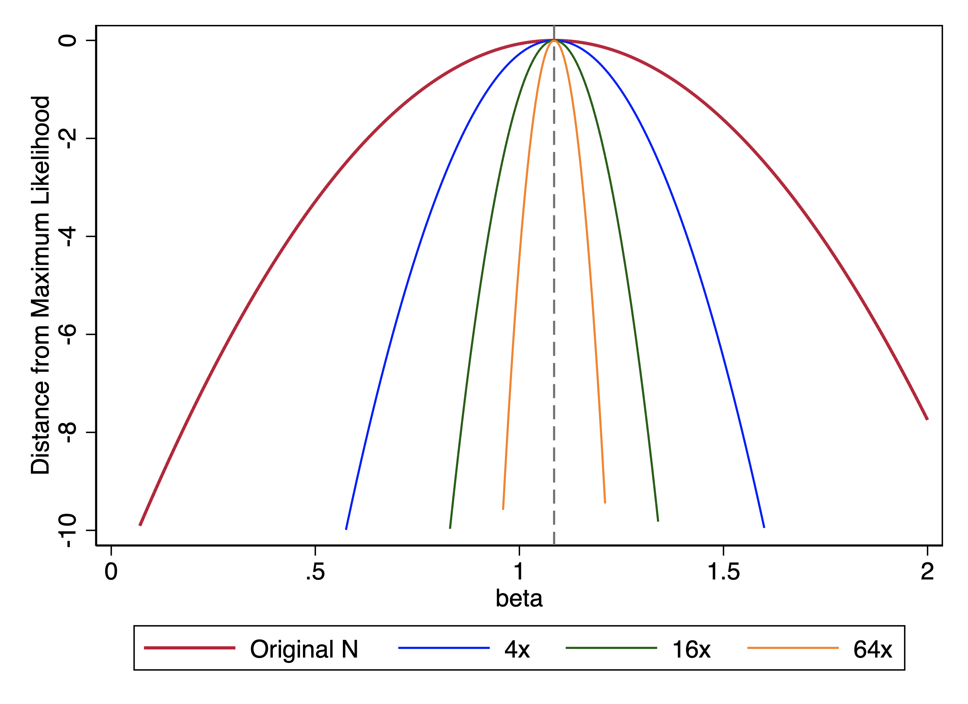
We noted how the sample that was 64x larger had a much steeper likelihood function than the original sample. Whenever we quadruple our sample size, we make the likelihood function twice as narrow.
With the likelihood ratio test, we fit two different models – our unconstrained model and a constrained model – and we compare the difference in their likelihoods. You can think about the above plot as showing what happens when you impose a constraint that \(\beta\) is a specific value rather than letting it take whatever value maximizes the likelihood. In this case, the plot illustrates that a steeper likelihood function means a bigger difference between the log-likelihoods of the constrained and unconstrained models.
A Wald test gets at the same idea but only fits one model (the unconstrained model). Rather than comparing two models, the Wald test looks at the curve of the likelihood function that it has fit.
There are a couple different ways of doing this, but the most intuitive involves what is called the Hessian. In statistics, the Hessian is a matrix of second-order partial derivatives, but we are not presuming that you know what that means. A second-order derivative reflects whether and how much the change in a function is accelerating or decelerating vs. changing at a steady rate. The steeper the likelihood function, the more rapid the deceleration as it approaches the maximum, and the more rapid the acceleration on its way back downhill past the maximum.
Aside: Why “Hessian”? Outside of statistics, a Hessian is a person from the German state of Hesse. The Hessian matrix is named after a particular German, Ludwig Hesse. (Come to think of it, my own surname is like Hesse insofar as it also derives from an area of Germany, Frisia.)
Even for a simple example, working through the calculation of the Wald test statistic would take us too far down the rabbit hole for our purposes. That said, in the case of the Wald test statistic for a single coefficient, we can say that:
\(W = \left(\frac{\hat{\beta_x}}{se(\hat{\beta_x})}\right)^2\)
or the square of the coefficient divided by its standard error, which can then be evaluated using a chi-squared distribution with 1 df.
(This way of explaining it is basically a cheat, as it takes the things I would need to work through to properly explain the Wald test and sneaks it into how the standard error is calculated, which is then just taken for granted. But going through all that would take us too far afield.)
When both the LR and Wald test are proper to use, they are asymptotically equal to one another. This means that if we had an infinitely large sample, the test statistics would be the same. Since we never have an infinitely large sample, the test statistics for Wald and LR will differ somewhat, although they will usually give the same substantive conclusion.
Sometimes when you have a choice in analyses it makes sense to do things both ways so you can see whether the choice makes a difference. That doesn’t really make sense here, so I would recommend just picking one and going with it.
When LR and Wald may both be used, there are some folks who will say that it does not make much difference which of the two one chooses, and there are other folks who will prefer the likelihood-ratio test. Why might one prefer the likelihood-ratio test?
We are not going to get into the details of robust standard errors here, but there are many cases in which you may choose to use them. More to the point, even when you are not explicitly choosing robust standard errors, things like using weights or clustered observations will cause Stata to use them automatically. In those cases, you will not be able to use a likelihood-ratio test and will have to use a Wald test.
Using the Titanic data, let’s compare the same model fit with and without robust standard errors, as it is telling:
Without robust standard errors:
df <- read_dta("../dta/titanic_passengers.dta")

# change reference category to category 3
df <- df %>%
  mutate(pclass = relevel(as_factor(pclass), ref = "3rd"),
         male = as_factor(male),
         child = as_factor(child))

# logit model without robust standard errors
model1 <- glm(survived ~ pclass + male + child, data = df, family = "binomial")
tula(model1)
Family: binomial / Link: logit
AIC = 1244.587 Number of obs = 1309
BIC = 1270.472 McFadden R-sq = 0.2909
Log likelihood = -617.293 Nagelkerke R-sq = 0.4362
─────────────────────────────────────────────────────────────────────────────
survived │ Coef Std. Err. z P>|z| [95% Conf Interval]
─────────────────────────────────────────────────────────────────────────────
pclass │
1st │ 1.862 .1761 10.57 <.0001 1.517 2.207
2nd │ .8977 .1802 4.981 <.0001 .5445 1.251
male │ -2.499 .1484 -16.84 <.0001 -2.79 -2.208
child │ 1.085 .2292 4.735 <.0001 .636 1.535
(Intercept) │ .2047 .1287 1.59 .1119 -.04766 .457
─────────────────────────────────────────────────────────────────────────────. logit survived ib3.pclass male child, nolog
Logistic regression Number of obs = 1,309
LR chi2(4) = 506.44
Prob > chi2 = 0.0000
Log likelihood = -617.29343 Pseudo R2 = 0.2909
------------------------------------------------------------------------------
survived | Coefficient Std. err. z P>|z| [95% conf. interval]
-------------+----------------------------------------------------------------
pclass |
1st | 1.861954 .1760938 10.57 0.000 1.516816 2.207091
2nd | .8976734 .1802103 4.98 0.000 .5444676 1.250879
|
male | -2.499297 .1483849 -16.84 0.000 -2.790126 -2.208467
child | 1.085262 .2292127 4.73 0.000 .636013 1.53451
_cons | .2046715 .1287436 1.59 0.112 -.0476614 .4570044
------------------------------------------------------------------------------
With robust standard errors:
# same model with robust standard errors
tula(model1, robust=TRUE)
Family: binomial / Link: logit
AIC = 1244.587 Number of obs = 1309
BIC = 1270.472 McFadden R-sq = 0.2909
Log likelihood = -617.293 Nagelkerke R-sq = 0.4362
─────────────────────────────────────────────────────────────────────────────
survived │ Coef Robust SE z P>|z| [95% Conf Interval]
─────────────────────────────────────────────────────────────────────────────
pclass │
1st │ 1.862 .1736 10.72 <.0001 1.522 2.202
2nd │ .8977 .1689 5.315 <.0001 .5667 1.229
male │ -2.499 .1463 -17.09 <.0001 -2.786 -2.213
child │ 1.085 .2602 4.17 <.0001 .5752 1.595
(Intercept) │ .2047 .1317 1.554 .1201 -.05343 .4628
─────────────────────────────────────────────────────────────────────────────. logit survived ib3.pclass male child, nolog robust Logistic regression Number of obs = 1,309 Wald chi2(4) = 343.51 Prob > chi2 = 0.0000 Log pseudolikelihood = -617.29343 Pseudo R2 = 0.2909 ------------------------------------------------------------------------------ | Robust survived | Coefficient std. err. z P>|z| [95% conf. interval] -------------+---------------------------------------------------------------- pclass | 1st | 1.861954 .1731023 10.76 0.000 1.522679 2.201228 2nd | .8976734 .1681295 5.34 0.000 .5681457 1.227201 | male | -2.499297 .1457393 -17.15 0.000 -2.78494 -2.213653 child | 1.085262 .2579969 4.21 0.000 .579597 1.590926 _cons | .2046715 .1311434 1.56 0.119 -.0523648 .4617078 ------------------------------------------------------------------------------
The coefficient estimates themselves are exactly the same across the two models. The standard errors are not, as robust standard errors are used in the second model.
In the Stata output, there is another difference, which is that when you use robust standard errors, Stata changes the label of the “log likelihood” of the model to the “log pseudolikelihood.” The actual value of the log-likelihood/pseudolikelihood is exactly the same; only the label has changed.
Stata is opinionated here: it takes the position that if robust standard errors are to be used, then the assumptions that would justify ordinary (aka “naive”) standard errors no longer apply. These assumptions are the same as those which would undergird using the likelihood for other purposes, like the likelihood-ratio test. So it considers it a contradiction to fit a model and ask for robust standard errors and then think it would be proper to use a likelihood-ratio test.
So Stata stamps “pseudolikelihood” on the output when robust standard errors are used. In addition:
R is less opinionated than Stata about this. R’s lrtest() function will happily perform a likelihood-ratio test regardless of whether you have used robust standard errors, without any warning or refusal. But it is probably better to follow Stata’s lead and not do so.
While many of our analyses that use the General Social Survey in this course do not use weights, if we were doing analyses for a paper we probably would use weights. We definitely want to use weights for simple descriptive statistics, although that intuition often leads people to overestimate how much weights will affect coefficient estimates in regression models.
Here is an example from the 2006 GSS using weights where our outcome is being a religious none and our explanatory variables are birth year, sex, and zodiac sign.
df <- read_dta("../dta/gss_norelig_thru2018.dta") %>%
  mutate(relig_none = norelig)

# filter to 2006 only
df_2006 <- df %>%
  filter(year == 2006) %>%
  drop_na(zodiac) %>%
  mutate(zodiac = as_factor(zodiac))

model <- glm(relig_none ~ cohort + as_factor(female) + zodiac,
             data = df_2006, weights = wtssall, family = "binomial")
Warning in eval(family$initialize): non-integer #successes in a binomial glm!tula(model, robust=TRUE)Family: binomial / Link: logit
AIC = 3362.853 Number of obs = 4332
BIC = 3452.086 McFadden R-sq = 0.03966
Log likelihood = -1667.427 Nagelkerke R-sq = 0.05837
────────────────────────────────────────────────────────────────────────────────
relig_none │ Coef Robust SE z P>|z| [95% Conf Interval]
────────────────────────────────────────────────────────────────────────────────
cohort │ .02598 .003115 8.341 <.0001 .01988 .03209
as_factor(fe~) │
female │ -.5122 .0988 -5.185 <.0001 -.7059 -.3186
zodiac │
taurus │ -.1216 .2303 -.5282 .5974 -.5731 .3298
gemini │ -.1685 .2213 -.7614 .4464 -.6024 .2653
cancer │ -.2017 .2258 -.8932 .3717 -.6443 .2409
leo │ -.4227 .238 -1.776 .0758 -.8892 .04386
virgo │ -.3575 .2258 -1.583 .1134 -.8001 .08513
libra │ -.1353 .2328 -.5811 .5612 -.5916 .321
scorpio │ -.5337 .2502 -2.133 .0329 -1.024 -.04338
sagittarius │ -.1654 .2357 -.7016 .4829 -.6274 .2966
capricorn │ -.5475 .2504 -2.187 .0288 -1.038 -.05678
aquarius │ -.09127 .2248 -.406 .6847 -.5318 .3493
pisces │ -.5796 .2328 -2.49 .0128 -1.036 -.1233
(Intercept) │ -52.16 6.114 -8.531 <.0001 -64.14 -40.17
────────────────────────────────────────────────────────────────────────────────. logit norelig cohort i.female i.zodiac [pweight = wtssall] if year == 2006, nolog
Logistic regression Number of obs = 4,332
Wald chi2(13) = 112.06
Prob > chi2 = 0.0000
Log pseudolikelihood = -1809.6199 Pseudo R2 = 0.0397
------------------------------------------------------------------------------
| Robust
norelig | Coefficient std. err. z P>|z| [95% conf. interval]
-------------+----------------------------------------------------------------
cohort | .0259833 .0030937 8.40 0.000 .0199197 .0320469
|
female |
female | -.5122256 .0981372 -5.22 0.000 -.7045709 -.3198803
|
zodiac |
taurus | -.1216483 .2287023 -0.53 0.595 -.5698966 .3266001
gemini | -.1685266 .2198578 -0.77 0.443 -.5994401 .2623868
cancer | -.2017239 .2244484 -0.90 0.369 -.6416348 .2381869
leo | -.4226783 .2365641 -1.79 0.074 -.8863355 .0409789
virgo | -.3574653 .2245115 -1.59 0.111 -.7974997 .0825692
libra | -.1352826 .2312431 -0.59 0.559 -.5885108 .3179456
scorpio | -.533742 .2483434 -2.15 0.032 -1.020486 -.0469979
sagittarius | -.1653792 .2341418 -0.71 0.480 -.6242887 .2935302
capricorn | -.5475448 .2482047 -2.21 0.027 -1.034017 -.0610724
aquarius | -.0912656 .2232037 -0.41 0.683 -.5287368 .3462055
pisces | -.5796138 .2315336 -2.50 0.012 -1.033411 -.1258162
|
_cons | -52.15819 6.072557 -8.59 0.000 -64.06018 -40.2562
------------------------------------------------------------------------------
Surprisingly, some coefficients for zodiac sign are statistically significant. Then again, is this that surprising? After all, there are 12 different zodiac signs, and 1 in 20 results are expected to be significant by chance alone. And we didn’t have any specific predictions about which zodiac signs would be related to being a religious none, even though we can always invent some post hoc explanation (e.g., Pisces were less likely than Aries to be religious nones; the Pisces symbol is fish; and fish has a special significance in the Christian religious tradition; so maybe Pisces really are more likely to be religious, at least relative to those sheeple Aries).
Instead, though, we may wish to test whether the zodiac coefficients are simultaneously equal to zero, which is a joint hypothesis. If robust standard errors were not used, we could do this using a likelihood-ratio test. But because these estimates use weights, robust standard errors are used and Stata will not let us use a likelihood ratio test. We can still use a Wald test. (Note that even though the zodiac coefficients are labeled in the output, we cannot use these labels but have to refer to the categories as \(\texttt{2.zodiac}\) .. \(\texttt{12.zodiac}\), where \(\texttt{1.zodiac}\) (Aries) is the reference category.)
# test whether zodiac signs are jointly zero
hypothesis <- c("zodiactaurus = 0",
                "zodiacgemini = 0",
                "zodiaccancer = 0",
                "zodiacleo = 0",
                "zodiacvirgo = 0",
                "zodiaclibra = 0",
                "zodiacscorpio = 0",
                "zodiacsagittarius = 0",
                "zodiaccapricorn = 0",
                "zodiacaquarius = 0",
                "zodiacpisces = 0")

linearHypothesis(model, hypothesis, vcov = vcovHC(model, type = "HC1")) # uses "car" library
Linear hypothesis test:
zodiactaurus = 0
zodiacgemini = 0
zodiaccancer = 0
zodiacleo = 0
zodiacvirgo = 0
zodiaclibra = 0
zodiacscorpio = 0
zodiacsagittarius = 0
zodiaccapricorn = 0
zodiacaquarius = 0
zodiacpisces = 0

Model 1: restricted model
Model 2: relig_none ~ cohort + as_factor(female) + zodiac

Note: Coefficient covariance matrix supplied.

  Res.Df Df  Chisq Pr(>Chisq)
1   4329
2   4318 11 14.803     0.1917
. test 2.zodiac 3.zodiac 4.zodiac 5.zodiac 6.zodiac ///
>         7.zodiac 8.zodiac 9.zodiac 10.zodiac 11.zodiac 12.zodiac

 ( 1)  [norelig]2.zodiac = 0
 ( 2)  [norelig]3.zodiac = 0
 ( 3)  [norelig]4.zodiac = 0
 ( 4)  [norelig]5.zodiac = 0
 ( 5)  [norelig]6.zodiac = 0
 ( 6)  [norelig]7.zodiac = 0
 ( 7)  [norelig]8.zodiac = 0
 ( 8)  [norelig]9.zodiac = 0
 ( 9)  [norelig]10.zodiac = 0
 (10)  [norelig]11.zodiac = 0
 (11)  [norelig]12.zodiac = 0

           chi2( 11) =   14.85
         Prob > chi2 =    0.1896
The \(p\)-value for the joint test is \(.18\), and so the brief hopes of a positive astrological finding have been dashed.
Parental education predicts whether a child grows up to be a religious none. But is mother’s or father’s education more predictive in this regard?
We can fit a logit model with mother’s (maeduc) and father’s (paeduc) education (measured in years) as explanatory variables:
model <- glm(relig_none ~ paeduc + maeduc, data = df, family = "binomial")
tula(model)
Family: binomial / Link: logit
AIC = 29881.033 Number of obs = 42603
BIC = 29907.012 McFadden R-sq = 0.0247
Log likelihood = -14937.517 Nagelkerke R-sq = 0.03433
─────────────────────────────────────────────────────────────────────────────
relig_none │ Coef Std. Err. z P>|z| [95% Conf Interval]
─────────────────────────────────────────────────────────────────────────────
paeduc │ .05879 .00495 11.88 <.0001 .04909 .06849
maeduc │ .06224 .005998 10.38 <.0001 .05048 .074
(Intercept) │ -3.417 .05867 -58.24 <.0001 -3.532 -3.302
─────────────────────────────────────────────────────────────────────────────. logit norelig paeduc maeduc, nolog
Logistic regression Number of obs = 42,603
LR chi2(2) = 756.57
Prob > chi2 = 0.0000
Log likelihood = -14937.517 Pseudo R2 = 0.0247
------------------------------------------------------------------------------
norelig | Coefficient Std. err. z P>|z| [95% conf. interval]
-------------+----------------------------------------------------------------
paeduc | .0587891 .0049501 11.88 0.000 .049087 .0684912
maeduc | .0622405 .0059982 10.38 0.000 .0504842 .0739969
_cons | -3.416869 .0586712 -58.24 0.000 -3.531862 -3.301876
------------------------------------------------------------------------------
From this, we can see that both coefficients are statistically significant, and also that the coefficient for \(\texttt{maeduc}\) is larger than the coefficient for \(\texttt{paeduc}\). But, is the difference between \(\texttt{maeduc}\) and \(\texttt{paeduc}\) statistically significant?
In principle, one could test this using a likelihood-ratio test by fitting a constrained model in which the coefficients for \(\texttt{maeduc}\) and \(\texttt{paeduc}\) were constrained to be equal, and then comparing the likelihood of that model to the likelihood of the unconstrained model. However, it is easier to test this using a Wald test.
In R, we can use the linearHypothesis function from the car package:
# test equality of paeduc and maeduc coefficients
linearHypothesis(model, "paeduc = maeduc")
Linear hypothesis test:
paeduc - maeduc = 0

Model 1: restricted model
Model 2: relig_none ~ paeduc + maeduc

  Res.Df Df  Chisq Pr(>Chisq)
1  42601
2  42600  1 0.1207     0.7283
In Stata, the command for a Wald test is \(\texttt{test}\).
. test paeduc = maeduc

 ( 1)  [norelig]paeduc - [norelig]maeduc = 0

           chi2(  1) =    0.12
         Prob > chi2 =    0.7283
From this result, we conclude that we do not have any evidence that there is a difference between mother’s education and father’s education.