Expand to show code to load packages
# dependencies
library(tidyverse)
library(tulaverse)
library(haven)We have been talking about how to interpret and present estimates from the logit model. What we have postponed until now, however, is talking about where these estimates come from in the first place.
When we fit the linear regression model using OLS, estimates are those that minimize the sum of squared residuals. That’s what least squares (the LS in OLS) is.
The logit model is not fit using OLS. After all, if we took the residual \(\hat{y} - y\) when y is a binary outcome and minimized the sum of squares of that, we would be back at the linear probability model.
Instead, we fit the logit model using maximum likelihood estimation.
Here is our first pass at the big idea of maximum likelihood:
Maximum likelihood estimates are the \(\beta\textrm{'s}\) for which the outcome values we observed are most likely, given the values of the explanatory variables.
We have already seen how the logit model allows us to calculate the predicted probability of both \(y=1\) and \(y=0\). Our maximum likelihood estimates are the estimates that maximize the predicted probabilities of observing the values of the outcome that were actually observed.
That is, we will select the \(\mathbf{\beta}\) that:
We are going to walk through an example with the logit model.
In our example, we are going to look at passenger data from the Titanic.
Let’s introduce five passengers in these data, who we will follow through this example.
# dependencies
library(tidyverse)
library(tulaverse)
library(haven)data <- read_dta("../dta/titanic_passengers.dta") %>%
mutate(child = as_factor(child, levels = "labels")) %>%
mutate(female = as_factor(female, levels = "labels")) %>%
mutate(pclass = as_factor(pclass, levels = "labels")) %>%
mutate(survived = as_factor(survived, levels = "labels")) %>%
mutate(pclass = relevel(pclass, ref="3rd"))
data %>%
arrange(name) %>%
filter(row_number() >= 906 & row_number() <= 910) %>%
select(name, female, child, pclass, survived)# A tibble: 5 × 5
name female child pclass survived
<chr> <fct> <fct> <fct> <fct>
1 Oreskovic, Mr. Luka male adult 3rd died
2 Osen, Mr. Olaf Elon male child 3rd died
3 Osman, Mrs. Mara female adult 3rd survived
4 Ostby, Miss. Helene Ragnhild female adult 1st survived
5 Ostby, Mr. Engelhart Cornelius male adult 1st died . list name female child pclass survived in 906/910, noobs +---------------------------------------------------------------------+ | name female child pclass survived | |---------------------------------------------------------------------| | Oreskovic, Mr. Luka male adult 3rd died | | Osen, Mr. Olaf Elon male child 3rd died | | Osman, Mrs. Mara female adult 3rd survived | | Ostby, Miss. Helene Ragnhild female adult 1st survived | | Ostby, Mr. Engelhart Cornelius male adult 1st died | +---------------------------------------------------------------------+
Helene Ostby and Mara Osman both survived; they were adult women sailing in first and third class respectively. The other three died: Engelhart Ostby, a man in 1st class; Luka Oreskovic, a man in 3rd class; and Olaf Osen, a child in 3rd class.
We fit our logit model:
model <- glm(survived ~ female + child + pclass,
             data = data, family = "binomial")
tula(model)
Family: binomial / Link: logit
AIC = 1244.587 Number of obs = 1309
BIC = 1270.472 McFadden R-sq = 0.2909
Log likelihood = -617.293 Nagelkerke R-sq = 0.4362
─────────────────────────────────────────────────────────────────────────────
survived │ Coef Std. Err. z P>|z| [95% Conf Interval]
─────────────────────────────────────────────────────────────────────────────
female │ 2.499 .1484 16.84 <.0001 2.208 2.79
child │ 1.085 .2292 4.735 <.0001 .636 1.535
pclass │
1st │ 1.862 .1761 10.57 <.0001 1.517 2.207
2nd │ .8977 .1802 4.981 <.0001 .5445 1.251
(Intercept) │ -2.295 .1353 -16.96 <.0001 -2.56 -2.029
─────────────────────────────────────────────────────────────────────────────. logit survived i.female i.child ib3.pclass
Iteration 0: log likelihood = -870.51219
Iteration 1: log likelihood = -622.08358
Iteration 2: log likelihood = -617.30582
Iteration 3: log likelihood = -617.29343
Iteration 4: log likelihood = -617.29343
Logistic regression Number of obs = 1,309
LR chi2(4) = 506.44
Prob > chi2 = 0.0000
Log likelihood = -617.29343 Pseudo R2 = 0.2909
------------------------------------------------------------------------------
survived | Coef. Std. Err. z P>|z| [95% Conf. Interval]
-------------+----------------------------------------------------------------
1.female | 2.499297 .1483849 16.84 0.000 2.208467 2.790126
1.child | 1.085262 .2292127 4.73 0.000 .636013 1.53451
|
pclass |
1st | 1.861954 .1760938 10.57 0.000 1.516816 2.207091
2nd | .8976734 .1802103 4.98 0.000 .5444676 1.250879
|
_cons | -2.294625 .1352986 -16.96 0.000 -2.559805 -2.029445
------------------------------------------------------------------------------
The signs of these coefficients mean that women, children, and those with first and second class tickets were more likely to survive than men, adults, and those with third class tickets.
Notice the reported log-likelihood of \(-617.293\). Below, we are going to show how these estimates yield a log-likelihood of \(-617.293\).
When fitting a model using maximum likelihood, the software actually does its work in terms of the log-likelihood rather than the likelihood itself.
Because the above estimates are the maximum likelihood estimates, changing any of the \(\beta\) coefficients would make the log-likelihood worse (farther from zero) than \(-617.293\).
To begin, for every observation, we will calculate the predicted probability of survival. In the logit model, \(\Pr(y=1) = \frac{\exp(\mathbf{x}\mathbf{\beta})}{\exp(\mathbf{x}\mathbf{\beta}) + 1}\) . We will also calculate the probability of not surviving, which is \(1-\Pr(y=1)\).
data <- data %>%
  mutate(xbeta = predict(model)) %>%
  mutate(pr1 = predict(model, type="response")) %>%
  mutate(pr0 = 1 - pr1)

data %>%
  arrange(name) %>%
  filter(row_number() >= 906 & row_number() <= 910) %>%
  select(name, survived, xbeta, pr1, pr0) %>%
  mutate(across(where(is.double), ~round(., 4)))
# A tibble: 5 × 5
name survived xbeta pr1 pr0
<chr> <fct> <dbl> <dbl> <dbl>
1 Oreskovic, Mr. Luka died -2.29 0.0916 0.908
2 Osen, Mr. Olaf Elon died -1.21 0.230 0.770
3 Osman, Mrs. Mara survived 0.205 0.551 0.449
4 Ostby, Miss. Helene Ragnhild survived 2.07 0.888 0.112
5 Ostby, Mr. Engelhart Cornelius died -0.433 0.394 0.606. predict xbeta, xb . gen pr1 = exp(xbeta) / (1 + exp(xbeta)) // could have just said -predict, pr1- . gen pr0 = 1 - pr1 . format %6.4f pr1 pr0 xbeta // format so that it looks nice when listed . list name survived xbeta pr1 pr0 in 906/910, noobs +-----------------------------------------------------------------------+ | name survived xbeta pr1 pr0 | |-----------------------------------------------------------------------| | Oreskovic, Mr. Luka died -2.2946 0.0916 0.9084 | | Osen, Mr. Olaf Elon died -1.2094 0.2298 0.7702 | | Osman, Mrs. Mara survived 0.2047 0.5510 0.4490 | | Ostby, Miss. Helene Ragnhild survived 2.0666 0.8876 0.1124 | | Ostby, Mr. Engelhart Cornelius died -0.4327 0.3935 0.6065 | +-----------------------------------------------------------------------+
Stata: For illustrative purposes, we compute \(\mathbf{x}\mathbf{\beta}\) for the passengers first and then calculate the probability of survival given \(\mathbf{x}\mathbf{\beta}\), but we could have just done this in one step in Stata: \(\mathtt{predict pr1}\).
We can see above that poor Luka Oreskovic down in 3rd class had an \(\mathbf{x}\mathbf{\beta}\) of -2.2946. Exponentiating this yields an odds of \(\exp(-2.2946) = .10080\), which means that Pr(survival) for Luka was \(.10080/1.10080 = .0916\). And if Luka only had a 9.16% chance of surviving (\(y=1\)), this means he had a 90.84% chance of dying (\(y=0\)).
We are specifically interested in the predicted probability of what actually happened in each case. That is, we want the predicted probability of survival for those who survived and the predicted probability of dying for those who perished.
data <- data %>%
  mutate(pr_obs = ifelse(survived == "survived", pr1, pr0))

data %>%
  arrange(name) %>%
  filter(row_number() >= 906 & row_number() <= 910) %>%
  select(name, survived, pr1, pr0, pr_obs) %>%
  mutate(across(where(is.double), ~round(., 4)))
# A tibble: 5 × 5
name survived pr1 pr0 pr_obs
<chr> <fct> <dbl> <dbl> <dbl>
1 Oreskovic, Mr. Luka died 0.0916 0.908 0.908
2 Osen, Mr. Olaf Elon died 0.230 0.770 0.770
3 Osman, Mrs. Mara survived 0.551 0.449 0.551
4 Ostby, Miss. Helene Ragnhild survived 0.888 0.112 0.888
5 Ostby, Mr. Engelhart Cornelius died 0.394 0.606 0.606. gen pr_observed = pr1 if survived == 1
(809 missing values generated)
. replace pr_observed = pr0 if survived == 0
(809 real changes made)
. format %6.4f pr_observed
. list name survived pr1 pr0 pr_observed in 906/910, noobs abbrev(12)
+---------------------------------------------------------------------------+
| name survived pr1 pr0 pr_observed |
|---------------------------------------------------------------------------|
| Oreskovic, Mr. Luka died 0.0916 0.9084 0.9084 |
| Osen, Mr. Olaf Elon died 0.2298 0.7702 0.7702 |
| Osman, Mrs. Mara survived 0.5510 0.4490 0.5510 |
| Ostby, Miss. Helene Ragnhild survived 0.8876 0.1124 0.8876 |
| Ostby, Mr. Engelhart Cornelius died 0.3935 0.6065 0.6065 |
+---------------------------------------------------------------------------+
For the three passengers above who died, \(\Pr(\mathrm{observed})\) is the predicted probability that \(y=0\). For the two who survived, \(\Pr(\mathrm{observed})\) is the predicted probability that \(y=1\).
These values of \(\Pr(\mathrm{observed})\) are our likelihoods. As we noted before, instead of working with likelihoods, software works with log-likelihoods. So let’s compute the log-likelihoods for our five folks:
data <- data %>%
  mutate(ln_lik = log(pr_obs))

data %>%
  arrange(name) %>%
  filter(row_number() >= 906 & row_number() <= 910) %>%
  select(name, pr_obs, ln_lik) %>%
  mutate(across(where(is.double), ~round(., 4)))
# A tibble: 5 × 3
name pr_obs ln_lik
<chr> <dbl> <dbl>
1 Oreskovic, Mr. Luka 0.908 -0.096
2 Osen, Mr. Olaf Elon 0.770 -0.261
3 Osman, Mrs. Mara 0.551 -0.596
4 Ostby, Miss. Helene Ragnhild 0.888 -0.119
5 Ostby, Mr. Engelhart Cornelius 0.606 -0.5 . list name survived pr_observed ln_likelihood in 906/910, noobs abbrev(13)
+-------------------------------------------------------------------------+
| name survived pr_observed ln_likelihood |
|-------------------------------------------------------------------------|
| Oreskovic, Mr. Luka died 0.9084 -.0960364 |
| Osen, Mr. Olaf Elon died 0.7702 -.2611229 |
| Osman, Mrs. Mara survived 0.5510 -.5960386 |
| Ostby, Miss. Helene Ragnhild survived 0.8876 -.1192152 |
| Ostby, Mr. Engelhart Cornelius died 0.6065 -.5000318 |
+-------------------------------------------------------------------------+
As you can see, log-likelihoods are always negative. Of our five passengers, Luka Oreskovic, who died and had a 90.8% chance of dying, has the log-likelihood that is highest (closest to 0). Mara Osman, who had only a 55% chance of survival but did survive, has the lowest Pr(observed) of our five passengers, and so the lowest log-likelihood.
Now we want the total log-likelihood summed over all 1,309 passengers:
sum(data$ln_lik)[1] -617.2934. quietly sum ln_likelihood . display r(sum) -617.29343
Scroll back and you can see this sum, -617.2934, matches the reported log-likelihood of our model that we fit with logit.
What did we just do? Three steps:
And again, because our estimates are the maximum likelihood estimates, this means that any other set of possible estimates for our coefficients would have a worse (farther from zero) log-likelihood than -617.29343.
Elaboration: There is nothing mysterious about this quantity -617.29343. It’s just the sum of the log-likelihoods of our 1,309 observations. If we divide -617.29343 by 1,309, we get -.47158. Take the exponent of that, we get \(\exp(-.47158)\) = .6240. This is the mean predicted probability of the observed outcome. In other words, on average, whatever happened to each person on the Titanic had a 62.4% chance of happening, given our model estimates.
Logs turn multiplication problems into addition problems, because: \[ a \times b = \exp\left[\ln(a) + \ln(b)\right] \] When facing an arduous multiplication problem, then, one shortcut may be to use logs and convert the problem into an easier addition problem. This is why software works in terms of log-likelihoods instead of likelihoods.
In our example, we computed the log-likelihood for each observation and added them together. We could have used the likelihoods instead, but then we would have had to multiply rather than add — a much more difficult computational task.
Aside: Likelihoods are really small. That we are working with log-likelihoods can disguise how small they actually are. Consider our example, in which the log-likelihood of our estimates is \(-617.29343\). If we take the exponent of \(-617.29343\), we get the likelihood, which is \(.8182 \times 10^{-268}\).
The way you can think about this number is to imagine being on the Titanic as it struck the iceberg, and armed with our estimates and information on each passenger’s values for our explanatory variables, guessing whether they were going to survive or not. The likelihood then is our probability of guessing correctly for every one of the 1,309 passengers.
Back when we discussed least squares, we showed an example where we generated estimates iteratively: that is, we tried out different candidate estimates and saw which one minimized least squares.
OLS regression estimates may be obtained analytically. That is, there is a set of matrix algebra operations that the computer can perform to arrive at the estimates.
When a model is fit using maximum likelihood, this is not what is done. Instead, it is fit iteratively.
The software tries a set of candidate estimates, evaluates the likelihood, then tries another set to see whether it improves. It continues until it can no longer find an improvement, and those are the estimates.
The software is smart in how it does this. The analogy I use is to imagine being blindfolded, placed on a hill, and asked to find the top of the hill. You can feel the direction of the slope beneath your feet, and so you can walk uphill. Once you reach a spot that is flat and everywhere around you is downhill, you have reached the top.
(To extend the analogy, if the slope beneath you is steep, then you know you aren’t close to the top of the hill yet. As it starts to get flatter, you know the top of the hill is getting closer. When the software evaluates the likelihood, it also evaluates the gradient of the likelihood function at that point, and that gradient does not just tell it the direction for the next candidate estimates but also how far away from the current estimates the next guess should be—it will take smaller steps for its guesses as the surface flattens.)
To illustrate, let’s look at a continuous variable in the Titanic dataset, \(\mathtt{fare10}\), the price of a passenger’s fare (measured here in tens of dollars).
calculate_loglik <- function(beta_intercept, beta_fare10, data) {

  # calculate linear predictor
  linear_pred <- beta_intercept + beta_fare10 * data$fare10
  # calculate probabilities
  predictions <- exp(linear_pred) / (1 + exp(linear_pred))
  pr_observed <- ifelse(data$survived=="survived", predictions, 1-predictions)
  # calculate log-likelihood
  log_pr_observed <- log(pr_observed)

  return(sum(log_pr_observed, na.rm = TRUE))
}

beta_candidates <- seq(0, .2, by = 0.01)

log_liks <- sapply(beta_candidates, function(b) {
  calculate_loglik(-.8824, b, data)
})

results_df <- tibble(
  beta_fare10 = beta_candidates,
  log_likelihood = log_liks
)ggplot(results_df, aes(x = beta_fare10, y = log_likelihood)) +
geom_line(color = "red3", linewidth = 1) +
labs(x = "Candidate Beta Value for fare10",
y = "Log-Likelihood") +
theme_tula() +
theme(axis.text = element_text(size=12))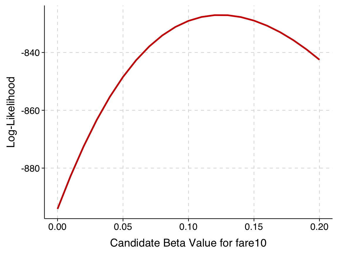
Zooming in (note the difference in axis scales):
beta_candidates <- seq(.11, .14, by = 0.001)
log_liks <- sapply(beta_candidates, function(b) {
calculate_loglik(-.8824, b, data)
})
results_df <- tibble(
beta_fare10 = beta_candidates,
log_likelihood = log_liks
)
ggplot(results_df, aes(x = beta_fare10, y = log_likelihood)) +
  geom_line(color = "red3", linewidth = 1) +
  labs(x = "Candidate Beta Value for fare10",
       y = "Log-Likelihood") +
  theme_tula() +
  theme(axis.text = element_text(size=12))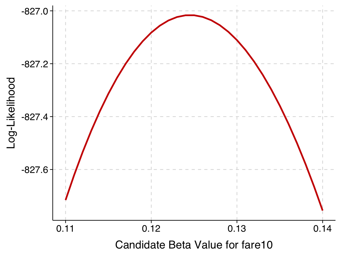
We can try different estimates of beta, calculate the log-likelihood, and see which maximizes the likelihood.
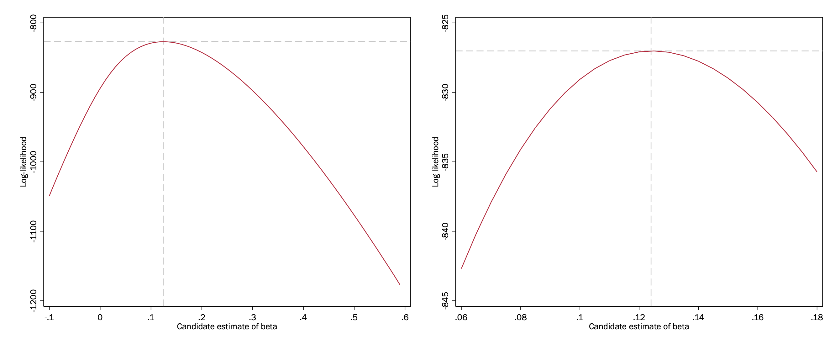
On the left, we try a broad range of beta values, and then on the right we zero in on a narrower range.
We can see from this that the best log-likelihood is between -825 and -830 for a \(\beta\) between .12 and .13. We can now fit the logit model using \(\texttt{logit}\) and confirm:
. logit survived fare10

Iteration 0:   log likelihood = -870.03074
Iteration 1:   log likelihood = -827.20729
Iteration 2:   log likelihood = -827.01611
Iteration 3:   log likelihood = -827.01595
Iteration 4:   log likelihood = -827.01595

Logistic regression                             Number of obs     =      1,308
                                                LR chi2(1)        =      86.03
                                                Prob > chi2       =     0.0000
Log likelihood = -827.01595                     Pseudo R2         =     0.0494

------------------------------------------------------------------------------
    survived |      Coef.   Std. Err.      z    P>|z|     [95% Conf. Interval]
-------------+----------------------------------------------------------------
      fare10 |   .1245273   .0160434     7.76   0.000     .0930828    .1559717
       _cons |  -.8824265   .0755229   -11.68   0.000    -1.030449   -.7344044
------------------------------------------------------------------------------
Aside: In reality, even in this simplest example there are two parameters–the \(\texttt{fare10}\) coefficient and the constant–but we are going to simplify this by magically assuming we know the correct answer for the constant and just changing the coefficient. But we could readily find the maximum likelihood for two different parameters at once; it’s just harder to visualize.
Here is a contour plot in R, where the peak of the hill is where the maximum likelihood estimates are:
# create sequences of candidate values for both parameters
beta_intercept_candidates <- seq(-.92, -0.84, by = 0.001)
beta_fare10_candidates <- seq(0.11, 0.14, by = 0.001)

# empty matrix to store log-likelihood values
log_lik_matrix <- matrix(NA,
                         nrow = length(beta_intercept_candidates),
                         ncol = length(beta_fare10_candidates))

# log-likelihood for each combination of parameters
for (i in 1:length(beta_intercept_candidates)) {
  for (j in 1:length(beta_fare10_candidates)) {
    log_lik_matrix[i, j] <- calculate_loglik(beta_intercept_candidates[i],
                                             beta_fare10_candidates[j],
                                             data)
  }
}

# fit model so we can place point on plot
actual_model <- glm(survived ~ fare10, data = data, family = binomial())
actual_intercept <- coef(actual_model)[1]
actual_fare10 <- coef(actual_model)[2]

# convert to data frame for ggplot
log_lik_df <- expand.grid(
  beta_intercept = beta_intercept_candidates,
  beta_fare10 = beta_fare10_candidates
)
log_lik_df$log_likelihood <- as.vector(log_lik_matrix)

# Create contour plot
ggplot(log_lik_df, aes(x = beta_intercept, y = beta_fare10, z = log_likelihood)) +
  geom_contour_filled(bins = 15) +
  annotate("segment", x = actual_intercept, xend = actual_intercept,
           y = 0.11, yend = actual_fare10,
           color = "red3", linetype = "dashed", linewidth = 0.5) +
  annotate("segment", x = -0.92, xend = actual_intercept,
           y = actual_fare10, yend = actual_fare10,
           color = "red3", linetype = "dashed", linewidth = 0.5) +
  geom_point(aes(x = actual_intercept, y = actual_fare10, z = NULL),
             color = "red4", size = 3) +
  labs(
    x = "Intercept (β0)",
    y = "fare10 coefficient (β1)"
  ) +
  theme_tula() +
  theme(legend.position = "none")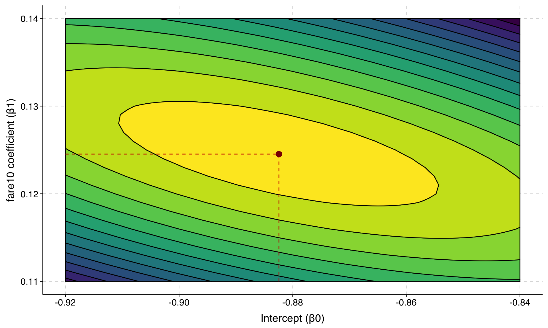
The deviance is equal to the log-likelihood multiplied by -2. In R, if you add control = glm.control(trace = TRUE) to the glm() function when you fit a model, R will provide the deviance for each iteration.
Here we can see this for the model of the Titanic data:
model <- glm(survived ~ female + child + pclass,
             data = data, family = "binomial",
             control = glm.control(trace = TRUE))
Deviance = 1239.676 Iterations - 1
Deviance = 1234.61 Iterations - 2
Deviance = 1234.587 Iterations - 3
Deviance = 1234.587 Iterations - 4R arrived at the estimates in 4 iterations. Because the deviance is the log-likelihood multiplied by -2, the deviance is always positive and lower deviance is better. If we divide the deviance of the final iteration by \(-2\), i.e., \(1234.59 / {-2}\), we get \(-617.29\), which is the log-likelihood of this model.
Let’s take another look at this part of the logit output that I just showed:
Iteration 0:   log likelihood = -870.03074
Iteration 1:   log likelihood = -827.20729
Iteration 2:   log likelihood = -827.01611
Iteration 3:   log likelihood = -827.01595
Iteration 4:   log likelihood = -827.01595
This shows Stata’s journey to finding the maximum likelihood estimates. Iteration 0 is its first guess. When evaluating a guess, it is looking at the slope of the hill at that guess, and it uses that to figure out a good next guess. You can see the log-likelihood at Iteration 1 is already close to the ultimate answer, showing how efficient this process of iteratively finding the maximum can be. (How does Stata know it’s found the maximum? When it’s landed on a spot on the hill that is flat.)
In Stata, if you specify \(\mathtt{trace}\) when fitting a maximum likelihood model, you can even eavesdrop on the specific guesses that Stata is evaluating at each iteration:
. logit survived fare10, trace

Iteration 0:
Parameter vector:
     survived:  survived:
       fare10      _cons
r1          0   -.479954

                                                   log likelihood = -870.03074
------------------------------------------------------------------------------------------------
Iteration 1:
Parameter vector:
     survived:  survived:
       fare10      _cons
r1   .1335872  -.9247389

                                                   log likelihood = -827.20729
------------------------------------------------------------------------------------------------
Iteration 2:
Parameter vector:
     survived:  survived:
       fare10      _cons
r1   .1242467  -.8816514

                                                   log likelihood = -827.01611
------------------------------------------------------------------------------------------------
Iteration 3:
Parameter vector:
     survived:  survived:
       fare10      _cons
r1   .1245269  -.8824258

                                                   log likelihood = -827.01595
------------------------------------------------------------------------------------------------
Iteration 4:
Parameter vector:
     survived:  survived:
       fare10      _cons
r1   .1245273  -.8824265

                                                   log likelihood = -827.01595