and the errors were distributed normally with a mean of 0 and standard deviation of 1.
The way that unobserved \(y^\ast\) mapped onto our observed binary variable was whether or not y* was greater than a threshold \(\tau\).
For ordered responses, we will follow the same principle. The key difference is that, instead of having one threshold \(\tau\), we will have \(k-1\) thresholds, where \(k\) is our number of categories.
As for how this maps onto the ordered variable we observe, imagine a survey item that has as its response categories: (1) strongly disagree (2) disagree (3) agree (4) strongly agree. We would have three thresholds: \(\tau_1\), \(\tau_2\), and \(\tau_3\). We would observe:
\(y =\) “strongly disagree” if \(y^\ast < \tau_1\)
\(y =\) “disagree” if \(y^\ast > \tau_1\) and \(y^\ast < \tau_2\)
\(y =\) “agree” if \(y^\ast > \tau_2\) and \(y^\ast < \tau_3\)
\(y =\) “strongly agree” if \(y^\ast > \tau_3\)
For purposes of estimation, all this needs to map onto the number line somehow.
In the binary probit model, we did this by constraining \(\tau\) to 0 because that made things simplest. But now that we have multiple thresholds, this is no longer the case.
Instead, what will is constrain the constant of our model (\(\beta_0\)) to be 0, and we will estimate values for the thresholds at the same time that we estimate our coefficients.
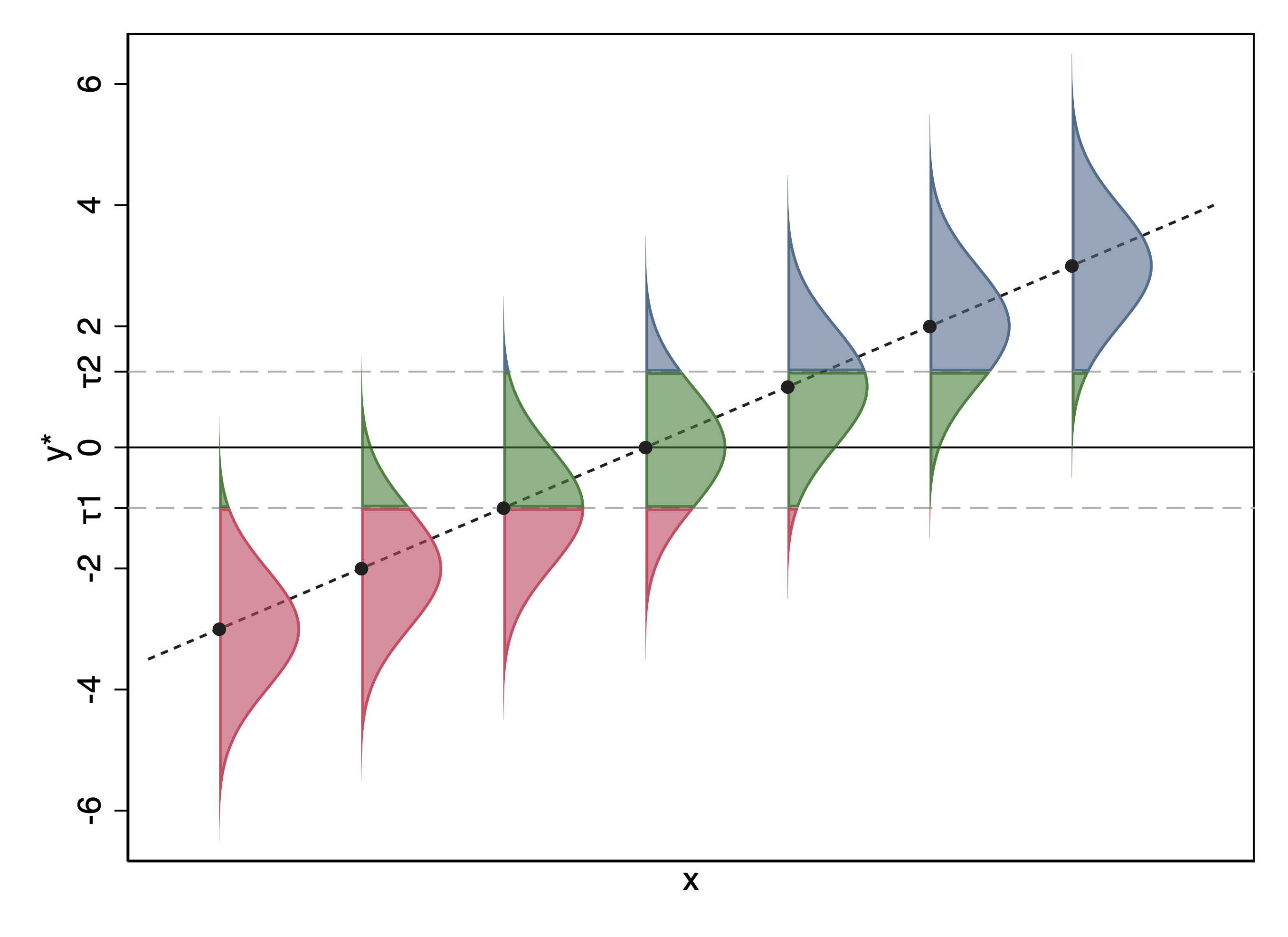
Here is a visualization of the ordered probit model for a three-category outcome.
In this visualization, notice that:
As x increases, the probability of the lowest (red) category decreases.
As x increases, the probability of the highest (blue) category increases.
As x increases, the probability of the middle (green) category first increases and then decreases.
For this middle category, whether the probability increases or decreases depends on whether more of the normal curve is shifting over \(\tau_1\) (thus entering from the lowest category) or shifting over \(\tau_2\) (thus exiting into the highest category)
Predicted probability of different outcomes
We will be able to fit our model using maximum likelihood so long as we have a means of computing the predicted probability of observing each of our outcome categories, for whatever value of \(\mathbf{x}\mathbf{\beta}\).
The math is easiest if we consider our \(k\) categories to be numbered as consecutive integers starting with 1.
We proceed again as in binary probit, by remembering that \(y^\ast = \mathbf{x}\mathbf{\beta} + \varepsilon\) and that \(\varepsilon\) is distributed as standard normal. Consequently, for a given value of \(\mathbf{x}\mathbf{\beta}\), the predicted probability will be based on what different random draws from \(\varepsilon\) result imply for \(\mathbf{x}\mathbf{\beta} + \varepsilon\) with respect to our thresholds.
For binary outcomes, the predicted probability that \(y = 1\) was \(\mathtt{cdf}_{\mathtt{normal}}(\mathbf{x}\mathbf{\beta} - \tau)\), where \(\mathtt{cdf}_{\mathtt{normal}}()\) is the cumulative distribution function of the standard normal distribution.
For ordered outcomes, we can follow the same reasoning to consider \(\Pr(y > m)\), where \(m\) is one of our categories. Then, \(\Pr(y > m) = \mathtt{cdf}_{\mathtt{normal}}(\mathbf{x}\mathbf{\beta}-\tau_m)\).
To make the math complete, we will add extra thresholds past the ends of our latent continuum:
\(\tau_0\) at \(-\infty\) so that \(\Pr(y > 0) = 1\)
\(\tau_k\) at \(\infty\) so that \(\Pr(y > k) = 0\)
Given that we can calculate \(\Pr(y > m)\) for any outcome, we can then calculate \(\Pr(y=m)\) for any outcome using subtraction:
Let’s demonstrate how predicted probabilities are calculated with an example. The General Social Survey starts with a battery of items asking respondents for their opinion about national spending in several domains. One is spending on “improving and protecting the nation’s health.” The response categories are: (1) too little, (2) about right, and (3) too much. We will consider this categorical variable as the observed manifestation of the underlying latent variable “opposition to government health care spending.”
We fit a simple model in which our explanatory variables are sex (measured as male/female) and political party (measured as Dem/Ind/Rep. We fit the model using the probit model for ordered responses, which in Stata can be fit using the \(\texttt{oprobit}\) command.
With the binary probit model, we said that we could have derived the binary logit model following the same reasoning with a couple twists. Specifically, instead of assuming the errors are normally distributed, we assumed they followed the logistic distribution, and instead of assuming the standard deviation of the error term is 1, we assume that it is \(\frac{\pi}{\sqrt{3}}\). We assume both these things because then and only then is the resulting model equivalent to what we developed earlier by writing a model in which the outcome was log odds.
If we make the same changes to the above model, we get what’s known as the ordered logit model instead of the ordered probit model. There’s a different way to get to the ordered logit model that is more directly in the spirit of logit as a log odds model, and so when we talk about it more it will be in that context.